
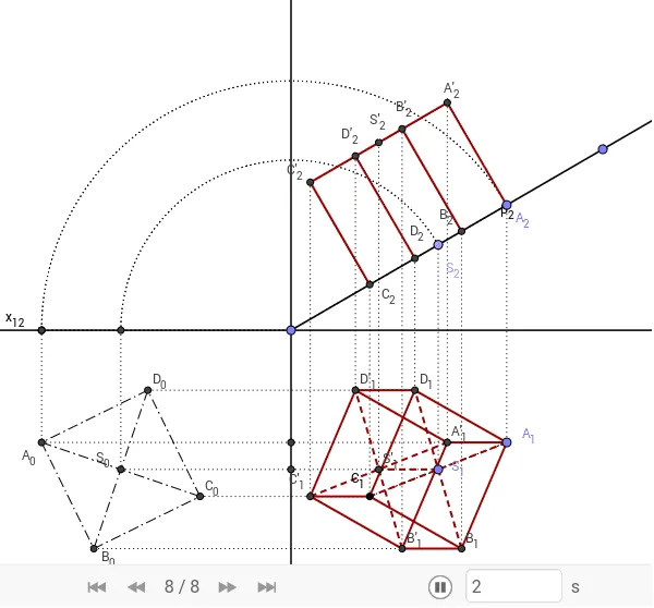
蒙日投影下的立方体
几何画板及绘图内容加载中,请稍等……
① 本范例演示如何利用蒙日投影(正交投影)得到立方体的俯视图与主视图,并已知某一面的平面、中心与顶点。② 涉及的核心数学概念包括立体几何中的正交投影、描述几何的蒙日投影原理、空间向量与平面的相对位置、以及投影变换的几何性质。③ 作图要点:使用 Point、Ray、OrthogonalLine、Segment、Mirror、Intersect、Line、Circle、CircleSector、CircleArc 等命令,构造点 x12、A、B、β2、S2、A2、b、c、S1、A1、d、e、C1、a、C2、f、a4、g、h、i、So、Ao、k、p、p3、A0、A02、r3、j、q3、S0、s3、F、G、c4、t3、l、C0、n、q 等对象,通过射线、垂线、线段、镜像、相交、圆弧等步骤完成两个投影面的构建。④ 适合高中立体几何、大学描述几何课程教学演示,也可作为几何作图训练与投影变换理解的教学素材。
GeoGebra 命令及参数
Point(x_{12}) → BRay(B, A) → β_2Point(β_2) → S_2Point(β_2) → A_2OrthogonalLine(S_2, x_{12}) → bOrthogonalLine(A_2, x_{12}) → cPoint(b) → S_1Point(c) → A_1Segment(S_2, S_1) → dSegment(A_2, A_1) → eMirror(A_1, S_1) → C_1OrthogonalLine(C_1, x_{12}) → aIntersect(a, β_2) → C_2Segment(C_1, C_2) → fSegment(A_1, C_1) → a_4Line(S_1, x_{12}) → gLine(A_1, x_{12}) → hOrthogonalLine(B, x_{12}) → iIntersect(g, i) → S_oIntersect(h, i) → A_oCircle(S_o, Segment[B, S_2]) → kCircle(A_o, Segment[B, A_2]) → pCircle(B, A_2) → p_3Intersect(p, h, 1) → A_0Intersect(p_3, x_{12}, 1) → A_{02}CircleSector(B, A_2, A_{02}) → r_3Segment(A_0, A_1) → jSegment(A_{02}, A_0) → q_3Intersect(k, g, 1) → S_0Circle(B, S_2) → s_3Intersect(s_3, x_{12}) → F, GCircleArc(B, S_2, F) → c_4Segment(F, S_0) → t_3Segment(S_0, S_1) → lMirror(A_0, S_0) → C_0Segment(A_0, C_0) → nOrthogonalLine(S_0, n) → qCircle(S_0, C_0) → rIntersect(r, q, 2) → D_0Intersect(r, q, 1) → B_0Segment(B_0, D_0) → sSegment(A_0, B_0) → tSegment(B_0, C_0) → a_1Segment(C_0, D_0) → b_1Segment(D_0, A_0) → c_1OrthogonalLine(B_0, i) → d_1Segment(C_0, C_1) → mOrthogonalLine(D_0, i) → e_1Intersect(i, e_1) → D_oIntersect(i, d_1) → B_oCircle(B, Segment[D_0, D_o]) → f_1Intersect(f_1, β_2, 1) → D_2OrthogonalLine(D_2, x_{12}) → g_1Intersect(e_1, g_1) → D_1Segment(D_0, D_1) → h_1Segment(D_1, D_2) → i_1Circle(B, Segment[B_0, B_o]) → k_1Intersect(k_1, β_2, 1) → B_2OrthogonalLine(B_2, x_{12}) → j_1Intersect(d_1, j_1) → B_1Segment(B_0, B_1) → l_1Segment(B_1, B_2) → m_1Segment(B_1, A_1) → n_1Segment(A_1, D_1) → p_1Segment(D_1, C_1) → q_1Segment(C_1, B_1) → r_1Segment(B_1, D_1) → s_1Segment(A_1, C_1) → t_1OrthogonalLine(C_2, β_2) → a_2OrthogonalLine(B_2, β_2) → b_2OrthogonalLine(S_2, β_2) → c_2OrthogonalLine(D_2, β_2) → d_2OrthogonalLine(A_2, β_2) → e_2Circle(S_2, Segment[A_0, B_0]) → f_2Intersect(f_2, c_2, 2) → S'_2OrthogonalLine(S'_2, c_2) → g_2Intersect(a_2, g_2) → C'_2Intersect(b_2, g_2) → B'_2Intersect(d_2, g_2) → D'_2Intersect(e_2, g_2) → A'_2Segment(C_2, C'_2) → h_2Segment(B_2, B'_2) → i_2Segment(D_2, D'_2) → j_2Segment(A_2, A'_2) → k_2Segment(A'_2, C'_2) → l_2OrthogonalLine(A'_2, x_{12}) → m_2OrthogonalLine(D'_2, x_{12}) → n_2OrthogonalLine(S'_2, x_{12}) → p_2OrthogonalLine(B'_2, x_{12}) → q_2OrthogonalLine(C'_2, x_{12}) → r_2Intersect(r_2, m) → C'_1Intersect(q_2, d_1) → B'_1Intersect(p_2, g) → S'_1Intersect(n_2, e_1) → D'_1Intersect(m_2, h) → A'_1Segment(C'_2, C'_1) → s_2Segment(B'_2, B'_1) → t_2Segment(S'_2, S'_1) → a_3Segment(D'_2, D'_1) → b_3Segment(A'_2, A'_1) → c_3Segment(D_1, D'_1) → d_3Segment(S_1, S'_1) → e_3Segment(C_1, C'_1) → f_3Segment(B_1, B'_1) → g_3Segment(A_1, A'_1) → h_3Segment(D'_1, C'_1) → i_3Segment(C'_1, B'_1) → j_3Segment(B'_1, A'_1) → k_3Segment(B'_1, D'_1) → l_3Segment(C'_1, A'_1) → m_3Segment(D'_1, A'_1) → n_3Intersect(r_3, x_{12}, 1) → CIntersect(r_3, x_{12}, 1) → DIntersect(r_3, s_3, 1) → E