
对数函数图像绘制与比较
几何画板及绘图内容加载中,请稍等……
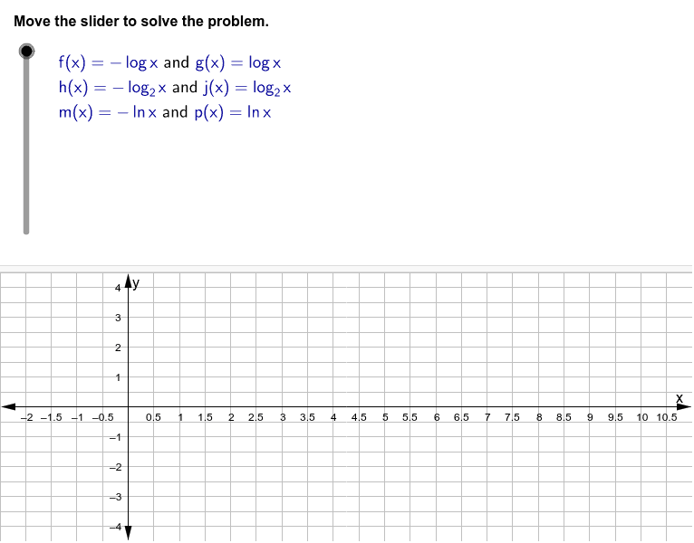
①本范例演示了三对对数函数的图像绘制与比较;②涉及核心数学概念包括对数函数的性质、图像平移、渐近线等;③作图要点使用了GeoGebra的Sequence, LaTeX, TableText, Ray, Text等命令和对象;④适合高中数学教学,用于理解函数图像变换与性质分析。
GeoGebra 命令及参数
Sequence(x = a, a, -7, -4, 0.5) → list1LaTeX("\textcolor{#000099}{f(x)=-\log x}\text{ and }\textcolor{#000099}{g(x)=\log x}") → pair1LaTeX("\textcolor{#000099}{h(x)=-\log_{2} {x}}\text{ and }\textcolor{#000099}{j(x)=\log_{2} {x}}") → pair2LaTeX("\text{Three pairs of logarithmic functions are provided. Graph each pair on one coordinate}\cr\text{plane. Then, use the graphs to identify and compare the asymptotes, intercepts,}\cr \text{domains, and ranges for each pair, as well as the shape and end behavior of each pair}\cr \text{of graphs.}") → problemtextLaTeX("\textcolor{#000099}{m(x)=-\ln x}\text{ and }\textcolor{#000099}{p(x)=\ln x}") → pair3TableText({{pair1}, {pair2}, {pair3}}, "l") → text1LaTeX("\text{Graph the first pair of functions on the same coordinate plane.}") → text2LaTeX("\textcolor{#FF0000}{f(x)=-\log x}") → ftextLaTeX("\textcolor{#006400}{g(x)=\log x}") → gtextLaTeX("\text{Compare the shapes and end behavior of the graphs.}") → text3LaTeX("\text{The line of reflection is the }\textcolor{#FF00FF}\text{x-axis}\text{.}") → text4LaTeX((((("\text{The shape and end behavior of the graph of }\textcolor{#FF0000}{" * ftext) * "}\text{ are inverted}\cr \text{from the shape and end behavior of the graph of }\textcolor{#006400}{") * gtext) * "}\text{. In}\cr \text{other words, the two graphs are reflections of each other.} ")) → text33LaTeX((((("\text{The graph of }\textcolor{#FF0000}{" * ftext) * "}\text{ decreases as }\textcolor{#000099}\text{x}\text{ approaches positive infinity.}\cr \text{The graph of }\textcolor{#006400}{") * gtext) * "}\text{ increases as }\textcolor{#000099}\text{x}\text{ approaches positive infinity.}")) → text5LaTeX("\text{Identify the two graphs’ asymptotes, intercepts, domains, and ranges.}") → text6LaTeX("\text{Since neither graph crosses the }\textcolor{#000099}\text{y-axis}\text{, both graphs have a vertical}\cr\text{asymptote at }\textcolor{#FF00FF}\text{x = 0}\text{.}") → text7LaTeX("\text{The graphs cross the }\textcolor{#000099}\text{x-axis}\text{ at the x-intercept }\textcolor{#000099}{\left(1, 0 \right)}\text{.}") → text8LaTeX("\text{Since the }\textcolor{#000099}{x-values}\text{ increase into positive infinity but never cross the}\cr\textcolor{#000099}{y-axis}\text{, this means they are never negative. Thus, we can determine the}\cr\text{domain of both graphs is }\textcolor{#000099}{x > 0}\text{.}") → text9Ray((0.1, 0), (1, 0)) → cLaTeX("\text{The range of both graphs is }{\textcolor{#000099}\text{all real numbers}\text{.}") → text10LaTeX("\text{Graph the second pair of functions together on a new coordinate plane.}") → text11LaTeX("\textcolor{#006400}{j(x)=\log_{2}{x}}") → jtextLaTeX("\textcolor{#FF0000}{h(x)=-\log_{2}{x}}") → htextLaTeX((((("\text{The graph of }\textcolor{#006400}{" * jtext) * "}\text{ and }\textcolor{#FF0000}{") * htext) * "}\text{ is shown.}")) → text111LaTeX("\text{Compare the shapes and end behavior of the second pair of graphs.}") → text12LaTeX((((("\text{The shape and end behavior of the graph of }{" * htext) * "}\text{ are inverted}\cr\text{from that of }{") * jtext) * "}\text{. In other words, each graph is a reflection of}\cr\text{the other over the }\textcolor{#FF00FF}\text{x-axis}\text{.}")) → text122LaTeX((((("\text{The graph of }{" * htext) * "}\text{ decreases as }\textcolor{#000099}\text{x}\text{ approaches positive infinity.}\cr \text{The graph of }{") * jtext) * "}\text{ increases as }\textcolor{#000099}\text{x}\text{ approaches positive infinity.}")) → text13LaTeX("\text{Identify the two graphs’ asymptotes, intercepts, domains, and ranges.}") → text14LaTeX("\text{There is a vertical asymptote at }{\textcolor{#FF00FF}\text{x = 0}\text{ for each graph.}") → text15LaTeX("\text{Both graphs cross the }\textcolor{#000099}\text{x-axis}\text{ at the x-intercept }\textcolor{#000099}{\left(1, 0\right)}\text{.}") → text16LaTeX("\text{The domain of both graphs is }\textcolor{#000099}\text{x > 0}\text{.}") → text17LaTeX("\text{Since the y-values are not limited, we can determine the range of each graph}\cr\text{is }\textcolor{#000099}\text{all real numbers}\text{.}") → text18LaTeX("\text{Graph the third pair of functions together on a new coordinate plane.}\cr \text{Compare the graphs’ shapes and end behavior.}") → text19LaTeX("\textcolor{#006400}{p(x)=\ln x}") → ptextLaTeX("\textcolor{#FF0000}{m(x)=-\ln x}") → mtextLaTeX((((("\text{The graph of }{" * ptext) * "}\text{ and }{") * mtext) * "}\text{ is shown.}")) → text20LaTeX((((("\text{The shape and end behavior of the graph of }{" * mtext) * "}\text{ are inverted}\cr \text{from that of }{") * ptext) * "}\text{; therefore, the graphs are reflections of one}\cr\text{another. The line of reflection is the }\textcolor{#FF00FF}\text{x-axis}\text{.}")) → text21LaTeX((((("\text{The graph of }{" * mtext) * "}\text{ decreases as }\textcolor{#000099}\text{x}\text{ approaches positive infinity.}\cr\text{The graph of }{") * ptext) * "}\text{ increases as }\textcolor{#000099}\text{x}\text{ approaches positive infinity.}")) → text22LaTeX((((("\text{Graph the given functions, }{" * ftext) * "}\text{ and }{") * gtext) * "}\text{, by hand or}\cr\text{using a graphing calculator. The result should resemble the following.}")) → textnew2LaTeX("\text{Use the graphs to identify the asymptotes, intercepts, domains, and}\cr \text{ranges of this third pair of functions.}") → text23LaTeX("\text{There is a vertical asymptote at }\textcolor{#FF00FF}\text{x = 0}\text{.}") → text24LaTeX("\text{The graphs cross the x-axis at the x-intercept }\textcolor{#000099}{\left(1, 0\right)}\text{.}") → text25LaTeX("\text{The domain of both graphs is }\textcolor{#000099}\text{x > 0}\text{.}") → text26LaTeX("\text{The range of both graphs is }\textcolor{#000099}\text{all real numbers}\text{.}") → text27LaTeX("\text{Summarize your findings.}") → text28LaTeX("\text{In summary, all three pairs of graphs have the same vertical asymptote}\cr\text{of }\textcolor{#FF00FF}\text{x = 0}\text{. In every case, the x-intercept is }\textcolor{#000099}{\left(1, 0\right)}\text{. The domain and range}\cr \text{for all three pairs are identical. The three pairs of functions}\cr\text{differ in the rate of increase or decrease as }\textcolor{#000099}\text{x}\text{ increases.}") → text29Text("Move the slider to solve the problem.") → text0
AI 绘图提示语参考
绘制三对对数函数的图像,并比较它们。第一对是 f(x)=-logx 和 g(x)=logx,它们关于x轴对称,在x=1处相交,垂直渐近线为x=0,定义域为x>0,值域为所有实数。第二对是 h(x)=-log2x 和 j(x)=log2x,同样关于x轴对称,具有相同的渐近线、交点和定义域、值域。第三对是 m(x)=-lnx 和 p(x)=lnx,也关于x轴对称,具有相同的渐近线、交点和定义域、值域。所有图像在x轴正半轴上增加或减少,且形状互为镜像。
以上提示语为根据原始绘图命令整理而来,仅供参考。