
线性回归可视化 - 残差平方和
几何画板及绘图内容加载中,请稍等……
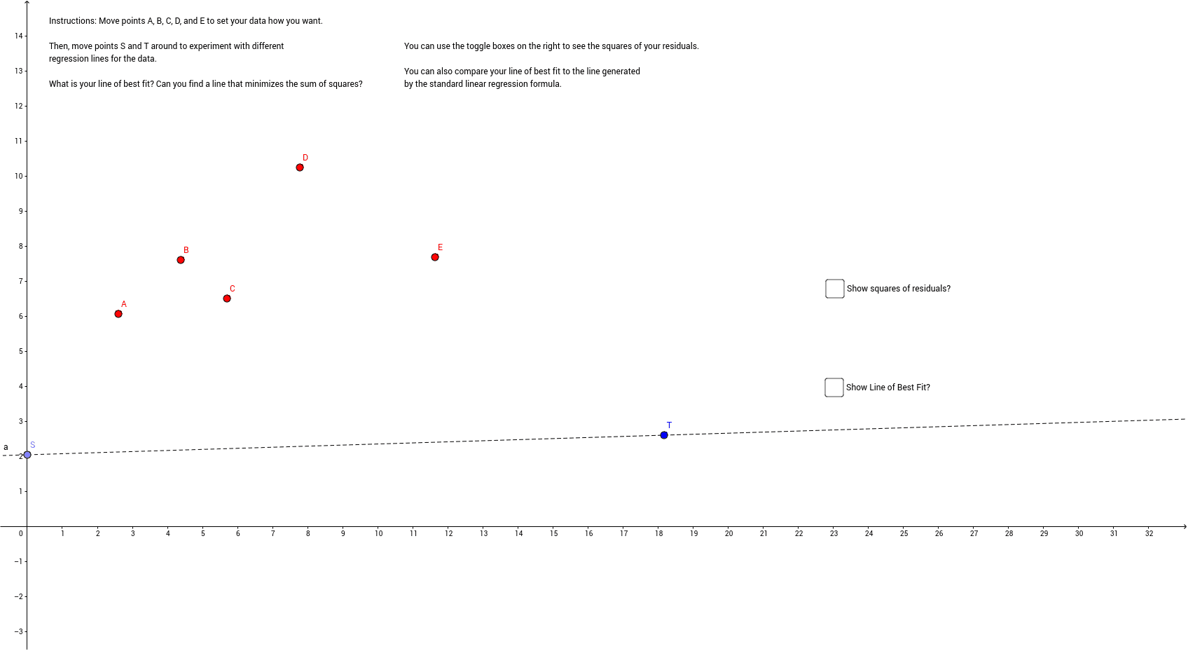
①本范例演示线性回归中残差平方和的计算与可视化;②涉及核心数学概念包括线性回归、残差平方和、最小二乘法;③作图要点:使用 GeoGebra 命令 Point, Line, OrthogonalLine, Intersect, Polygon, FitLineY, RSquare 构建数据点、回归线、残差等对象;④适合高中及以上数学学习者,用于理解线性回归模型评估指标。
GeoGebra 命令及参数
Point(yAxis) → SLine(S, T) → aOrthogonalLine(B, xAxis) → bOrthogonalLine(C, xAxis) → cOrthogonalLine(A, xAxis) → dOrthogonalLine(D, xAxis) → eOrthogonalLine(E, xAxis) → fIntersect(a, b) → HIntersect(d, a) → IIntersect(c, a) → JIntersect(a, e) → KIntersect(a, f) → LPolygon(H, B, 4) → poly1, g, h, i, j, M, NPolygon(I, A, 4) → poly2, k, l, m, n, O, PPolygon(J, C, 4) → poly3, p, q, r, s, Q, RPolygon(K, D, 4) → poly4, t, a_1, b_1, c_1, S_1, T_1Polygon(L, E, 4) → poly5, d_1, e_1, f_1, g_1, U, V_1FitLineY(DataSet) → h_1Intersect(h_1, b) → FIntersect(h_1, c) → GIntersect(h_1, d) → ZIntersect(h_1, e) → A_1Intersect(h_1, f) → B_1Polygon(F, B, 4) → poly6, i_1, j_1, k_1, l_1, C_1, D_1Polygon(G, C, 4) → poly7, m_1, n_1, p_1, q_1, E_1, F_1Polygon(Z, A, 4) → poly8, r_1, s_1, t_1, a_2, G_1, H_1Polygon(A_1, D, 4) → poly9, b_2, c_2, d_2, e_2, I_1, J_1Polygon(B_1, E, 4) → poly10, f_2, g_2, h_2, i_2, K_1, L_1RSquare({(-3, 2), (-2, 1), (-1, 3), (0, 4), (1, 2), (2, 4), (3, 3), (4, 5), (6, 4)}, (0.5 * x) + 2.5) → w