
绘制对数函数图像 by Walch Education
几何画板及绘图内容加载中,请稍等……
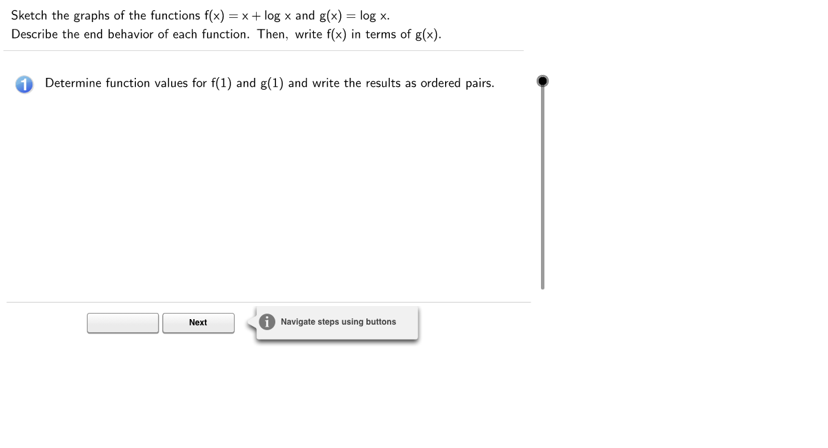
①本范例演示了在坐标系中绘制函数f(x) = x + log(x)和g(x) = log(x)的图像;②涉及的核心数学概念包括对数函数、函数图像绘制、坐标系;③作图要点使用了GeoGebra的If、LaTeX、FractionText命令以及对象如d、c、g、a、e、p、q、r、f、stepMax、hr、layer、stepper、steps、hotspot4、hr0、prevNext、prev、next、b、prevHotspot、nextHotspot、btnInfobox、b1、hr_{bottom}、b2、b3、b4、b5、b6、b7、btnsOGrandom、randomHotspot、ogHotspot、h、step1、step1_1、step1_2、s、rt;④适合高中数学教学,用于函数图像绘制与对比分析。
GeoGebra 命令及参数
If(d ≟ 1, " ", LaTeX[(d * "\cdot")]) → hLaTeX("\text{Determine function values for } f(1) \text{ and } g(1) \text{ and write the results as ordered pairs.}") → step1LaTeX("\text{Substitute } x = 1 \text{ into each function and solve.}") → step1_1LaTeX("\text{Write each as an ordered pair.}") → step1_2FractionText(s) → rtLaTeX("\text{Find the function value at which the functions are equal.}") → Xstep3XLaTeX(((((("\text{Substitute the approximate value of x from Step 2 into each function.} \cr\ \cr \cr\ \cr\ f(" * r) * ")\approx g(") * r) * ") \approx ") * s)) → Xstep3_1XLaTeX(((((("f(1) = " * d) * "+ \log (1) = ") * d) * " + 0 =") * d)) → step1_{11}LaTeX("g(1) = \log (1) = 0 ") → step1_{12}LaTeX("f(x) = g(x)") → step2_1LaTeX(" x=0") → step2_3LaTeX((" g(0.1) = \log \, (0.1) = " * g(0.1))) → step3_{g1}LaTeX((" g(1) = \log \, (1) = " * g(1))) → step3_{g2}LaTeX((" g(2) = \log \, (2) \approx " * g(2))) → step3_{g3}LaTeX((" g(3) = \log \, (3) \approx " * g(3))) → step3_{g4}LaTeX((" g(4) = \log \, (4) \approx " * g(4))) → step3_{g5}If(d ≟ 1, " ", LaTeX[d]) → h_2LaTeX((h_2 * "x + \log \, x = \log \, x")) → step2_2LaTeX("\text{Write f(x) in terms of g(x).}") → step5LaTeX("\text{Often functions are related, which can simplify graph sketching.}") → step5_1LaTeX("\text{Describe what happens to the function values for domain values less than 1.}") → step7LaTeX("\text{Find the value(s) of x at which f(x) = g(x). }\cr\text{This will reveal any point(s) of intersection, or solutions, of the system of equations.}") → step2LaTeX("\text{The value x=0 is not in the domain of these functions.} \cr\text{Therefore, there is no point of intersection or solution for f(x)= g(x).} ") → step2_4LaTeX("\text{Determine additional points for sketching the graph of each function.} ") → step3LaTeX((((((((("f(x) = " * h_2) * "x + \log \, x = ") * h_2) * " x + g(x) \text{ or } f(x) - g(x) = ") * h_2) * "x, \cr\text{which means the difference between the function values } \cr\text{at any value of x is } ") * h_2) * "x.")) → step5_2LaTeX("\text{Plot the graphs.}") → step6LaTeX("\text{Plot the graphs.}") → FormulaText["\text{Plot of the graphs.}"]LaTeX("\text{The graph indicates the function diverges, but the pattern is unclear.}") → step7_1LaTeX("\text{For g(x): The function values approach negative infinity as x approaches 0.} \cr\text{As x approaches 1, the function values converge on }0.") → step7_3LaTeX("\text{Describe what happens to the function values for domain values greater than 1.}") → step8LaTeX("\text{The graph indicates the function values increase, but the pattern is unclear.}") → step8_1LaTeX("\text{For g(x): The function values approach positive infinity as x increases } \cr\text{from x=1 to positive infinity. As x approaches 1 from the right, } \cr\text{the function values converge on }0.") → step8_3LaTeX((("\text{Sketch the graphs of the functions } f(x) = " * h_2) * " x + \log \,x \text{ and } g(x) = \log \,x. \cr\text{Describe the end behavior of each function. Then, write f(x) in terms of g(x).}")) → ProblemLaTeX((((((((" f(0.1) = " * h) * " (0.1)+ \log \, (0.1) = ") * h) * " 0.1 + (") * g(0.1)) * ") = ") * f(0.1))) → step3_{f1}LaTeX((((((((" f(1) = " * h) * " (1)+ \log \, (1) = ") * h) * " 1 + (") * g(1)) * ") = ") * f(1))) → step3_{f2}LaTeX((((((((" f(2) = " * h) * " (2)+ \log \, (2) = ") * h) * " 2 + (") * g(2)) * ") \approx ") * f(2))) → step3_{f3}LaTeX((((((((" f(3) = " * h) * " (3)+ \log \, (3) = ") * h) * " 3 + (") * g(3)) * ") \approx ") * f(3))) → step3_{f4}LaTeX((((((((" f(4) = " * h) * " (4)+ \log \, (4) = ") * h) * " 4 + (") * g(4)) * ") \approx ") * f(4))) → step3_{f5}LaTeX(" \text{Solve f(x) for x = 0.1, 1, 2, 3, and 4.}") → step3_{f}LaTeX(" \text{Solve g(x) for x = 0.1, 1, 2, 3, and 4.}") → step3_{g}LaTeX(((((((((((" \text{For } f(x): \cr\ A=(0.1, " * f(0.1)) * ") \cr\ B=(1, ") * f(1)) * ") \cr\ C=(2, ") * f(2)) * ") \cr\ D=(3,") * f(3)) * ") \cr\ E=(4,") * f(4)) * ") ")) → step4_1LaTeX(((((((((((" \text{For } g(x): \cr\ F=(0.1, " * g(0.1)) * ") \cr\ G=(1, ") * g(1)) * ") \cr\ H=(2, ") * g(2)) * ") \cr\ I=(3,") * g(3)) * ") \cr\ J=(4,") * g(4)) * ") ")) → step4_2LaTeX((("\text{For f(x): The function values approach negative infinity as x approaches 0.} \cr\text{As x approaches 1, the function values converge on }" * d) * ".")) → step7_2LaTeX((("\text{For f(x): The function values approach positive infinity as x increases } \cr\text{from x=1 to positive infinity. As x approaches 1 from the right, } \cr\text{the function values converge on }" * d) * ".")) → step8_2LaTeX((((("g(1) = " * g(1)) * ": (1, ") * g(1)) * ")")) → step1_{22}LaTeX((((("f(1) = " * d) * " : (1, ") * d) * ")")) → step1_{21}LaTeX("\text{Write and plot the additional points. Make sure to keep the points with the correct function.}") → step4
AI 绘图提示语参考
在坐标系中绘制函数 f(x) = x + log(x) 和 g(x) = log(x) 的图像,并标注关键点。首先计算 f(1) 和 g(1) 的值,然后找出函数相等的近似 x 值。接着,为两个函数计算并标注 x = 0.1, 1, 2, 3, 4 的函数值,绘制这些点并连线形成图像。最后,描述两个函数在接近 0 和趋向无穷大时的行为趋势,并分析 f(x) 与 g(x) 的关系。
以上提示语为根据原始绘图命令整理而来,仅供参考。