
定积分可视化演示(I)
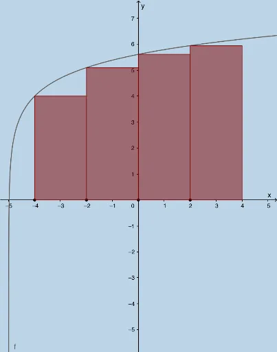
几何画板及绘图内容加载中,请稍等……
① 本范例通过动态图形直观展示定积分的几何意义,即函数曲线与x轴围成的面积,并利用矩形逼近(左和、右和)来近似积分值。② 核心数学概念包括定积分、黎曼和、极限思想、函数图像、区间划分以及面积计算。③ 作图要点:使用GeoGebra命令如Textfield创建输入框,Sequence生成分割点,Translate平移矩形,LeftSum和Sum计算左/右黎曼和,Intersect求交点,Polygon构造矩形,Integral直接绘制积分区域;涉及对象包括函数f、区间端点a、b、分割数n、矩形高度、中点、左右端点、矩形和等。④ 适合高中至大学低年级微积分教学,用于帮助学生理解定积分定义、黎曼和逼近过程以及积分与面积的关系,也可用于探究分割数n对逼近精度的影响。
GeoGebra 命令及参数
Textfield(f) → InputBox1Textfield(a) → InputBox2Textfield(b) → InputBox3Sequence((a + (i * deltax), 0), i, 1, n, 1) → rightxSequence((a + (i * deltax), f(a + (i * deltax))), i, 1, n, 1) → fofrightxSequence((a + (i * deltax), 0), i, 0, n - 1, 1) → leftxSequence(Midpoint[Element[leftx, i], Element[rightx, i]], i, 1, n, 1) → midpointsSequence((a + (i * deltax), f(a + (i * deltax))), i, 1, n, 1) → list1Translate(list1, (deltax, 0)) → list1'LeftSum(f, a, b, n) → lSequence(x = x(Element[midpoints, i]), i, 1, n, 1) → list2Sequence(Intersect[f, Element[list2, i], (3, 6.079441541679836)], i, 1, n, 1) → list3Translate(list3, (deltax / 2, 0)) → midpointtoprightTranslate(list3, (((-deltax)) / 2, 0)) → midpointtopleftTranslate(midpoints, (deltax / 2, 0)) → midpoints'Translate(midpoints, (((-deltax)) / 2, 0)) → midpoints'_1Sequence(Polygon[Element[midpoints'_1, i], Element[midpoints', i], Element[midpointtopright, i], Element[midpointtopleft, i]], i, 1, n, 1) → list4Sum(list4) → hTranslate(list1, ((-deltax), 0)) → list1'_1Translate(rightx, ((-deltax), 0)) → rightx'Sequence(Polygon[Element[rightx, i], Element[list1, i], Element[list1'_1, i], Element[rightx', i]], i, 1, n, 1) → rightrectanglesumSum(rightrectanglesum) → jIntersect(k, p) → FIntersect(m, k) → GPolygon(D, E, G, F) → poly1, d_1, e, g_1, f_1Intersect(m, q) → HIntersect(p, q) → IPolygon(D, E, H, I) → poly2, d_2, e_1, h_1, i_1Intersect(p, r) → JIntersect(r, m) → KPolygon(D, E, K, J) → poly3, d_3, e_2, k_1, j_1Integral(f, a, b) → s