
临界点作为几何中位数及其性质利用Hessian矩阵
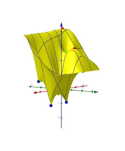
几何画板及绘图内容加载中,请稍等……
①本范例演示了如何通过GeoGebra绘制并分析函数的临界点作为几何中位数的性质;②涉及的核心数学概念包括临界点、Hessian矩阵、几何中位数、函数优化;③作图要点——使用了Polygon, PointIn, First, Sum, Sequence, Zip, TableText, Function, Length, Flatten, Textfield等命令和对象来构建图形和计算;④适合大学数学专业学生或对函数优化和几何性质感兴趣的学习者。
GeoGebra 命令及参数
Polygon({((-π), ((-π)) / 2), ((-π), π / 2), (π, π / 2), (π, ((-π)) / 2)}) → qPointIn(q) → aP1PointIn(q) → aP2PointIn(q) → aP3PointIn(q) → aP4PointIn(q) → aP5PointIn(q) → aP6PointIn(q) → aP7PointIn(q) → aP8PointIn(q) → P9PointIn(q) → aP10First({P1, P2, P3, P4, P5, P6, P7, P8, P9, P10}, n) → lPPointIn(q) → A_2Sum(Zip[sqrt((x(a) - ((R * cos(x)) * cos(y)))^(2) + (y(a) - ((R * sin(x)) * cos(y)))^(2) + (z(a) - (R * sin(y)))^(2)), a, lP]) → fSequence(If[D(i) > 0, If[f_{xx}(i) > 0, "local minimum", "local maximum"], If[(D(i) * f_{xx}(i)) ≟ 0, "?", "saddle point"]], i, 1, Length[l1]) → l4Zip((x(a), y(a)), a, l1) → l5TableText(Append["i", 1…Length[l1]], Append["critical points", l5], Append["f_{x}", lfx], Append["f_{y}", lfy], Append["f_{xx}", f_{xx}], Append["Det", D], Append["", l4], "v") → text1Function((q_f * f(u, v)) + b_0, u, (-π), π, v, ((-π)) / 2, π / 2) → f0Length(lsad) → läsadLength(lmax) → lämaxLength(lmin) → läminZip(Segment[A, p], p, lP) → segSum(seg) → sum_segFlatten(Sequence[Sequence[((-π) + ((2 * π / na) * i), ((-π)) / 2 + (π / na * j)), j, 1, na - 1], i, 1, na - 1]) → ltest_2Zip((R; x(a); y(a)), a, ltest_2) → ltest_3TableText(Append["i", Sequence[Length[lmax]]], Append["P_{Max }\;(φ,θ)", lmax], Append["(f'x,f'y)", lZf'xymax], "v") → textmaxTableText(Append["i", Sequence[Length[(lmin * x)]]], Append["P_{Max }\;(φ,θ)", lmin], Append["(f'x,f'y)", lZf'xymin], "v") → textminTableText(Append["i", Sequence[Length[(lsad * x)]]], Append["P_{Max }\;(φ,θ)", lsad], Append["(f'x,f'y)", lZf'xysad], "v") → textsadTextfield(R) → InputBox1Textfield(n) → InputBox2Textfield(lP0) → InputBox3