
Writing & Graphing Inequalities in GeoGebra: Visualizing the Solution Set
Loading the math board and drawing, please wait…
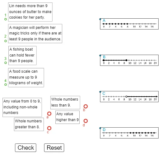
This example demonstrates how to translate inequality statements into geometric representations and visually identify the solution set. It focuses on the idea that the boundary (the equality case) separates the plane into regions, and the inequality selects which region(s) belong to the solution. Key concepts include inequality interpretation, geometric constraints, using distance-based or positional measures to decide membership, and distinguishing boundary vs. interior solutions. Construction details are reflected in the GeoGebra workflow: Zip and PolyLine are used to build key boundary/segmented graphical structures from multiple points (e.g., A, B, C, D, F, G, H, I, J, K, L). Distance-related quantities (given, adist, bdist, cdist, ddist, fdist and their variables) provide the computational basis for the inequality condition, while additional points/objects (M, N, O, P, Q, R and related entities) support the plotted geometry. The interface elements show and label the diagram (text1–text6, pic1, pic4), and buttons (button1, button2) guide step-by-step visualization. Suitable for middle school to high school math instruction, especially for linking algebraic inequalities with their graph-based interpretation.
GeoGebra Commands & Parameters
Zip(Distance[A, z], z, given) → adistZip(Distance[B, z], z, given) → bdistZip(Distance[C, z], z, given) → cdistZip(Distance[D, z], z, given) → ddistZip(Distance[F, z], z, given) → fdistPolyLine(Corner[pic1, 1], Corner[pic1, 2], Corner[pic1, 3], Corner[pic1, 4], Corner[pic1, 1]) → gPolyLine(Corner[pic4, 1], Corner[pic4, 2], Corner[pic4, 3], Corner[pic4, 4], Corner[pic4, 1]) → jPolyLine(Corner[text4, 1], Corner[text4, 2], Corner[text4, 3], Corner[text4, 4], Corner[text4, 1]) → lPolyLine(Corner[text3, 1], Corner[text3, 2], Corner[text3, 3], Corner[text3, 4], Corner[text3, 1]) → mPolyLine(Corner[text2, 1], Corner[text2, 2], Corner[text2, 3], Corner[text2, 4], Corner[text2, 1]) → nPolyLine(Corner[text1, 1], Corner[text1, 2], Corner[text1, 3], Corner[text1, 4], Corner[text1, 1]) → pZip(Distance[A, z], z, given2) → adist2Zip(Distance[B, z], z, given2) → bdist2Zip(Distance[C, z], z, given2) → cdist2Zip(Distance[D, z], z, given2) → ddist2PolyLine(Corner[pic2, 1], Corner[pic2, 2], Corner[pic2, 3], Corner[pic2, 4], Corner[pic2, 1]) → iPolyLine(Corner[pic3, 1], Corner[pic3, 2], Corner[pic3, 3], Corner[pic3, 4], Corner[pic3, 1]) → hPolyLine(Corner[text7, 1], Corner[text7, 2], Corner[text7, 3], Corner[text7, 4], Corner[text7, 1]) → kPolyLine(Corner[text8, 1], Corner[text8, 2], Corner[text8, 3], Corner[text8, 4], Corner[text8, 1]) → qPolyLine(Corner[text9, 1], Corner[text9, 2], Corner[text9, 3], Corner[text9, 4], Corner[text9, 1]) → rPolyLine(Corner[text10, 1], Corner[text10, 2], Corner[text10, 3], Corner[text10, 4], Corner[text10, 1]) → s
AI Drawing Prompt Reference
Draw a plane region graph defined by inequalities. First, draw boundary lines to represent equality conditions. Then, select interior or exterior regions based on the inequalities. Key objects include boundary points, region dividers, and labeled text. The construction order is to draw boundaries first, then determine regions based on inequalities, and finally add text labels to explain the graph.
The prompt above was compiled from the original drawing commands and is for reference only.