
Volumes by Cylindrical Shells
Loading the math board and drawing, please wait…
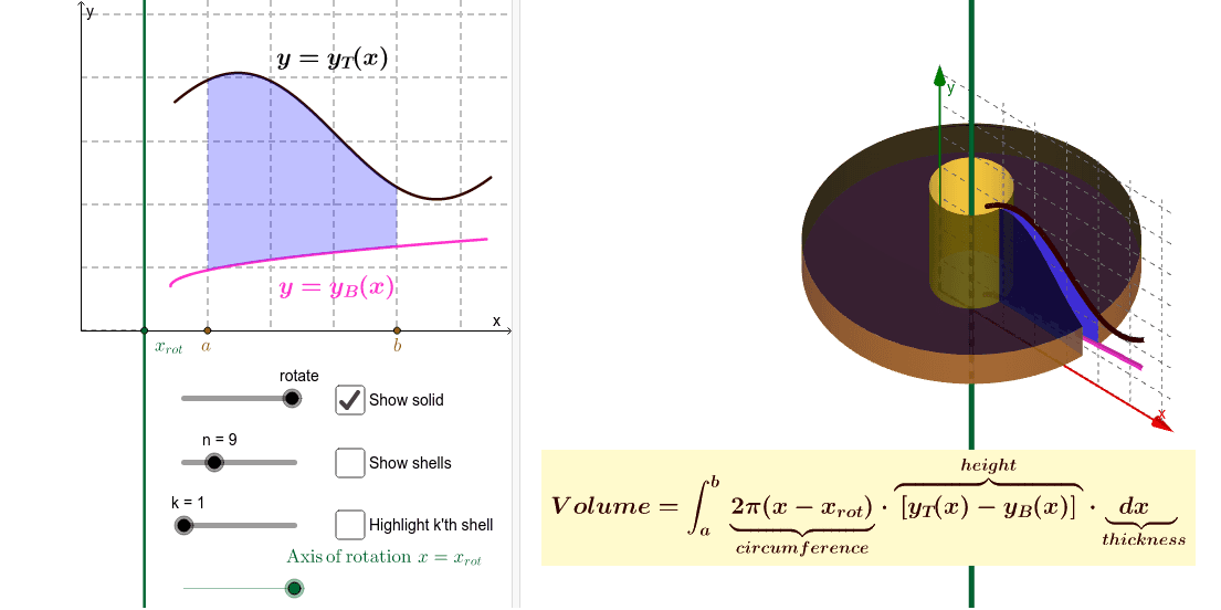
This example demonstrates how to calculate the volume of a solid of revolution using the method of cylindrical shells. Key concepts include integration, volume of solids of revolution, and the method of cylindrical shells. It constructs cylindrical shells, rotation axis, and regions to illustrate the geometric meaning of the method. Suitable for calculus courses.
GeoGebra Commands & Parameters
Sequence(a + ((k - 0.5) * dx), k, 1, n) → midptsSequence(a + (k * dx), k, 0, n - 1) → leftptsSequence(a + (k * dx), k, 1, n) → rightptsSequence(Polygon[(xk(k - 1), y_B(Element[evalpts, k])), (xk(k - 1), y_T(Element[evalpts, k])), (xk(k), y_T(Element[evalpts, k])), (xk(k), y_B(Element[evalpts, k]))], k, 1, n) → RectanglesSequence((Element[evalpts, k], 0), k, 1, n) → evalptsplotSurface(xrot + ((xk(k - 1) - xrot) * cos(t)), h, ((xk(k - 1) - xrot) * sin(t)), t, 0, (2 * π), h, y_B(Element[evalpts, k]), y_T(Element[evalpts, k])) → ShellIn_kSurface(xrot + (r * cos(t)), y_T(Element[evalpts, k]), (r * sin(t)), t, 0, (2 * π), r, xk(k - 1) - xrot, xk(k) - xrot) → UpShell_kSurface(xrot + ((xk(k) - xrot) * cos(t)), h, ((xk(k) - xrot) * sin(t)), t, 0, (2 * π), h, y_B(Element[evalpts, k]), y_T(Element[evalpts, k])) → ShellOut_kSurface(xrot + (r * cos(t)), y_B(Element[evalpts, k]), (r * sin(t)), t, 0, (2 * π), r, xk(k - 1) - xrot, xk(k) - xrot) → ShellDown_kSequence(Surface[xrot + ((xk(k - 1) - xrot) * cos(t)), h, ((xk(k - 1) - xrot) * sin(t)), t, 0, (2 * π), h, y_B(Element[evalpts, k]), y_T(Element[evalpts, k])], k, 1, n) → ShellsInSequence(Surface[xrot + (r * cos(t)), y_T(Element[evalpts, k]), (r * sin(t)), t, 0, (2 * π), r, xk(k - 1) - xrot, xk(k) - xrot], k, 1, n) → ShellsUpSequence(Surface[xrot + (r * cos(t)), y_B(Element[evalpts, k]), (r * sin(t)), t, 0, (2 * π), r, xk(k - 1) - xrot, xk(k) - xrot], k, 1, n) → ShellsDownSequence(Surface[xrot + ((xk(k) - xrot) * cos(t)), h, ((xk(k) - xrot) * sin(t)), t, 0, (2 * π), h, y_B(Element[evalpts, k]), y_T(Element[evalpts, k])], k, 1, n) → ShellsOutSurface(xrot + (cos((-t)) * (u - xrot)), y_B(u), (sin((-t)) * (u - xrot)), u, a, b, t, 0, RotationAngle) → Solid_BSurface(xrot + (cos((-t)) * (u - xrot)), y_T(u), (sin((-t)) * (u - xrot)), u, a, b, t, 0, RotationAngle) → Solid_TSurface(xrot + ((a - xrot) * cos((-t))), h, ((a - xrot) * sin((-t))), t, 0, RotationAngle, h, y_B(a), y_T(a)) → Solid_aSurface(xrot + ((b - xrot) * cos((-t))), h, ((b - xrot) * sin((-t))), t, 0, RotationAngle, h, y_B(b), y_T(b)) → Solid_bSurface(xrot + (cos((-RotationAngle)) * (u - xrot)), ((1 - w) * y_B(u)) + (w * y_T(u)), (sin((-RotationAngle)) * (u - xrot)), w, 0, 1, u, a, b) → Solid_eSurface(xrot + u - xrot, ((1 - w) * y_B(u)) + (w * y_T(u)), (0 * (u - xrot)), w, 0, 1, u, a, b) → region3dPolygon((xk(k - 1), y_B(Element[evalpts, k])), (xk(k - 1), y_T(Element[evalpts, k])), (xk(k), y_T(Element[evalpts, k])), (xk(k), y_B(Element[evalpts, k]))) → Rectangle_k, f, g, h, iSegment((0, 0), (xrot, 0)) → c
AI Drawing Prompt Reference
Draw a diagram illustrating the volume of a solid of revolution using the method of cylindrical shells. Start by drawing the rotation axis xrot, then draw a series of rectangles representing the bases of the cylindrical shells. Next, draw the cylindrical shells formed by rotating these rectangles around the axis, including both inner and outer shells. Finally, draw the boundaries of the solid, including the upper and lower boundaries.
The prompt above was compiled from the original drawing commands and is for reference only.