
Volume of Revolution Demo by Sébastien Vieilhescazes
Loading the math board and drawing, please wait…
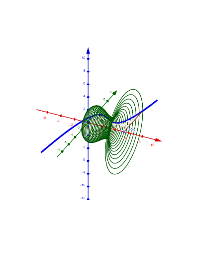
① This example demonstrates the generation of a solid of revolution by rotating a planar curve around an axis and dynamically visualizes the volume computation. ② Core mathematical concepts include definite integrals, the volume‑of‑revolution formula, piecewise functions, conditional probability interpreted geometrically, ratios and dilation transformations. ③ Construction highlights: the commands Point, Intersect, Line, Append, Polygon, Circle, Sequence, Rotate, CurveCartesian build the base curve and rotated surface; objects ShowVolume, RotateSurface, n_points, f, A, B, a, E, liste1, poly1, C, c, Mesh_1, Mesh_2, list1, list2, poly1', d, F, b together render the volume display and mesh subdivision. ④ Suitable for high‑school calculus electives, introductory university calculus, and geometric modeling courses, serving as an interactive aid for teaching and exploring volumes of revolution.
GeoGebra Commands & Parameters
Point(xAxis) → BIntersect(yAxis, zAxis) → ALine(A, B) → aPoint(a) → EAppend((x(E), 0), Append[(0, 0), Sequence[((x(E) * q / n_{points}), f((x(E) * q / n_{points}))), q, 0, n_{points}]]) → liste1Polygon(liste1) → poly1Circle(a, C) → cSequence(Circle[((q * x(E) / Mesh_2), 0, 0), f((q * x(E) / Mesh_2)), x + (0 * z) = 0], q, 0, Mesh_2) → list2Sequence(CurveCartesian[t, (f(t) * cos(((2 * π) * q / Mesh_1))), (f(t) * sin(((2 * π) * q / Mesh_1))), t, 0, x(E)], q, 1, Mesh_1) → list1Rotate(poly1, ((2 * π) * RotateSurface), a) → poly1'CurveCartesian(t, (f(t) * cos(((2 * π) * RotateSurface))), (f(t) * sin(((2 * π) * RotateSurface))), t, 0, x(E)) → b