
Volume of a Rectangular Prism by Courtney
Loading the math board and drawing, please wait…
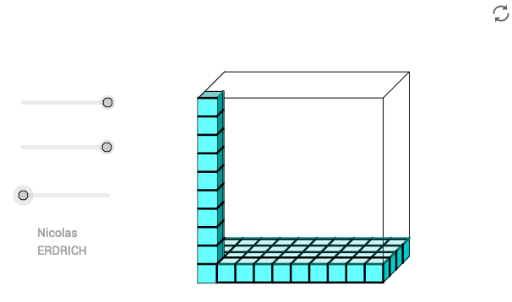
① This GeoGebra example dynamically displays a rectangular prism in 3D and computes its volume in real time, visually demonstrating the relationship between volume and the prism's length, width, and height. ② The core mathematical concept is the volume formula for a rectangular prism (V = length × width × height) in solid geometry, involving edges, faces, vertices, and volume measurement. ③ Construction highlights: from the construction summary, commands such as Line, OrthogonalLine, Circle, Intersect, Rotate, Angle, Segment, Midpoint, Polygon, Translate, Sequence, and Point are used to build the prism's framework, rotate the view, add auxiliary segments and labeled points, and form the solid surfaces via polygons poly1, poly2, poly3, with the volume stored in variable V. ④ Suitable for middle or high school solid geometry lessons, helping students grasp the geometric meaning of the volume formula and serving as an interactive tool for teachers to demonstrate volume calculation and spatial reasoning.
GeoGebra Commands & Parameters
Line(A, xAxis) → aOrthogonalLine(A, a) → q_4Circle(A, 2) → rIntersect(r, q_4, 2) → EIntersect(r, a, 2) → BOrthogonalLine(E, q_4) → sOrthogonalLine(B, a) → tIntersect(s, t) → FRotate(F, 45°, E) → S'Angle(F, E, S') → αSegment(E, S') → i_1Segment(E, F) → j_1Midpoint(j_1) → TCircle(E, T) → k_1Intersect(k_1, i_1, 1) → HSegment(E, H) → p_1Line(H, j_1) → q_1Line(F, p_1) → r_1Intersect(q_1, r_1) → VSegment(A, E) → s_1Segment(F, B) → t_1Line(B, r_1) → a_2Line(V, s_1) → b_2Intersect(a_2, b_2) → WPolygon(A, B, F, E) → poly1, p_2, r_2, s_2, q_2Polygon(B, W, V, F) → poly2, r_3, w, v, s_3Polygon(E, F, V, H) → poly3, q_3, s_4, v_1, uTranslate(A, B - A) → A'Translate(E, B - A) → E'Sequence(Sequence[Polygon[Translate[A, Vector[(k * Vector[A, B]) + (l * Vector[A, E])]], Translate[B, Vector[(k * Vector[A, B]) + (l * Vector[A, E])]], Translate[F, Vector[(k * Vector[A, B]) + (l * Vector[A, E])]], Translate[E, Vector[(k * Vector[A, B]) + (l * Vector[E, A])]]], k, 0, o], l, 0, 0) → ligneSequence(Sequence[Polygon[Translate[E, Vector[(l * Vector[A, B]) + (m * Vector[E, H])]], Translate[F, Vector[(l * Vector[A, B]) + (m * Vector[E, H])]], Translate[V, Vector[(l * Vector[A, B]) + (m * Vector[E, H])]], Translate[H, Vector[(l * Vector[A, B]) + (m * Vector[E, H])]]], l, 0, o], m, 0, q) → liste3Sequence(Polygon[Translate[B, (k * (W - B)) + (o * (B - A))], Translate[W, (k * (W - B)) + (o * (B - A))], Translate[V, (k * (W - B)) + (o * (B - A))], Translate[F, (k * (W - B)) + (o * (B - A))]], k, 0, q) → ligne2Sequence(Sequence[Polygon[Translate[A, Vector[(k * Vector[B, A]) - (l * Vector[E, A])]], Translate[B, Vector[(k * Vector[B, A]) - (l * Vector[E, A])]], Translate[F, Vector[(k * Vector[B, A]) - (l * Vector[E, A])]], Translate[E, Vector[(k * Vector[B, A]) - (l * Vector[E, A])]]], k, 0, 0], l, 0, p) → listeSequence(Sequence[Polygon[Translate[B, Vector[((-l) * Vector[E, A]) + (m * Vector[E, H])]], Translate[W, Vector[((-l) * Vector[E, A]) + (m * Vector[E, H])]], Translate[V, Vector[((-l) * Vector[E, A]) + (m * Vector[E, H])]], Translate[F, Vector[((-l) * Vector[E, A]) + (m * Vector[E, H])]]], l, 0, p], m, 0, 0) → liste2Translate(E, (p * (E - A))) → E'_1Translate(F, (p * (E - A))) → F'Translate(V, (p * (E - A))) → V'Translate(H, (p * (E - A))) → H'Polygon(E'_1, F', V', H') → Haut, e'_1, f', v', h'Translate(A, ((o + 1) * (B - A))) → Sommet1Translate(A, ((p + 1) * (E - A))) → Sommet2OrthogonalLine(E'_1, s_1) → bOrthogonalLine(Sommet1, p_2) → cIntersect(b, c) → Sommet3Translate(A, ((q + 1) * (H - E))) → Sommet4OrthogonalLine(Sommet4, p_2) → dSegment(A, Sommet4) → eSegment(A, E'_1) → fLine(E'_1, e) → gIntersect(d, g) → CLine(Sommet3, g) → hLine(C, b) → iIntersect(h, i) → DLine(D, d) → jLine(Sommet1, h) → kIntersect(j, k) → GSegment(E'_1, Sommet3) → lSegment(Sommet3, Sommet1) → mSegment(Sommet3, D) → nSegment(D, G) → a_1Segment(D, C) → b_1Segment(C, E'_1) → c_1Segment(F', B) → d_1Segment(V', V) → e_1Segment(H', V') → f_1Segment(A, Sommet1) → g_1Point(g_1) → ISegment(I, G) → h_1Segment(F, E) → l_1Segment(F, B) → m_1Line(E, g_1) → n_1Intersect(n_1, m) → JSegment(F, J) → c_2Segment(F', V') → d_2Segment(B, W) → e_2Line(J, h_1) → f_2Intersect(a_1, f_2) → KPoint(h_1) → LSegment(L, K) → g_2Segment(J, K) → h_2Line(H, h_1) → i_2Line(K, l) → j_2Intersect(i_2, j_2) → MSegment(M, K) → k_2Intersect(i_2, e_1) → NSegment(N, M) → l_2Intersect(r_1, j_2) → OSegment(F, O) → m_2Sequence(Segment[Translate[F, ((-k) * (A - B))], Translate[O, ((-k) * (A - B))]], k, 0, o) → seg4Line(N, b_1) → n_2Intersect(n_2, h_2) → PSegment(N, P) → t_2Line(V, t_2) → a_3Intersect(a_3, h_2) → QLine(S', a_3) → b_3Intersect(b_3, h_2) → RSegment(V, Q) → c_3Polygon(F, V, N, M, K, J) → poly4, f_3, v_2, n_3, m_3, k_3, j_3Polygon(V, F, F', V') → poly5, v_3, f_4, f'_1, v'_1Segment(N, M) → d_3Segment(M, K) → e_3Sequence(Segment[Translate[F, ((-k) * (A - E))], Translate[E, ((-k) * (A - E))]], k, 0, p) → seg_1Sequence(Segment[Translate[F, (k * (B - A))], Translate[B, (k * (B - A))]], k, 0, o) → seg_2Sequence(Segment[Translate[F, ((-l) * (E - H)) + (o * (B - A))], Translate[B, ((-l) * (E - H)) + (o * (B - A))]], l, 1, q) → seg10Sequence(Segment[Translate[N, (l * (H - E))], Translate[P, (l * (H - E))]], l, -2, q - 3) → seg5Sequence(Segment[Translate[B, ((-k) * (B - F))], Translate[W, ((-k) * (B - F))]], k, 1, p) → seg_3
AI Drawing Prompt Reference
Draw a rectangular prism with adjustable length, width, and height sliders. Start by creating a point A as one vertex of the prism, then create a line a through A and the x-axis. Next, create a circle r with radius 2 centered at A, and find its intersections with q_4 and a to get points B and E. Use rotations, angles, line segments, midpoints, and other operations to build the prism's framework, forming three base polygons poly1, poly2, and poly3. Finally, use translations and rotations to create the 3D structure of the prism and display its volume V.
The prompt above was compiled from the original drawing commands and is for reference only.