
Volume by Shells
Loading the math board and drawing, please wait…
In collections
AP Calculus volume problems
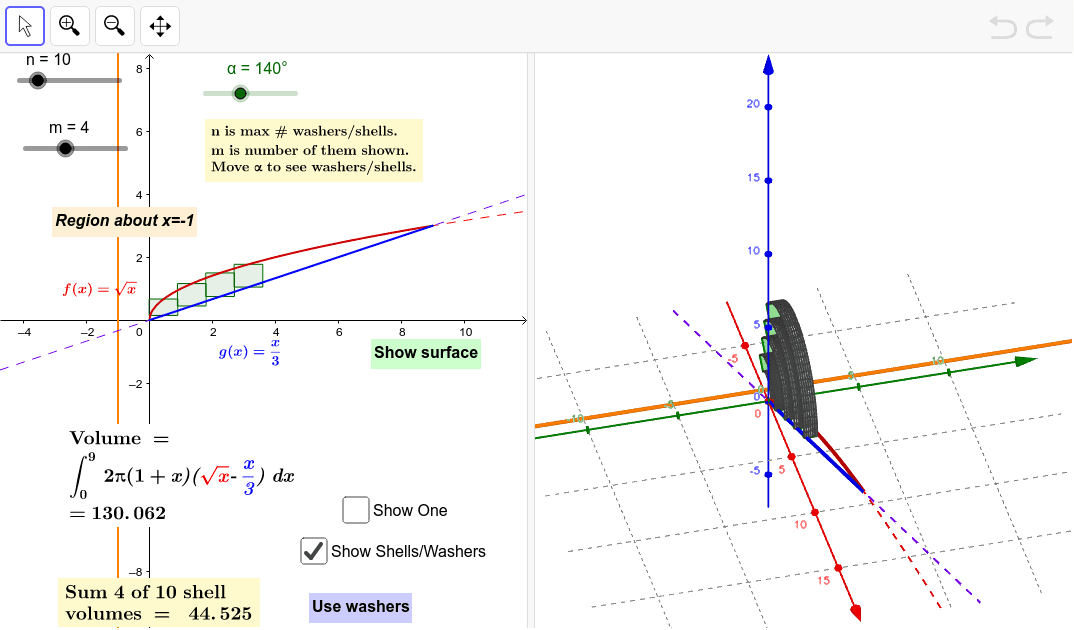
This example demonstrates a typical problem from the AP Calculus test, illustrating the calculation of the volume of a solid of revolution using integration. Key mathematical concepts include integration, volume of solids of revolution, and trigonometric functions. Using GeoGebra commands such as Sequence, Rotate, and Integral, the formation process of the solid of revolution is dynamically shown. Suitable for high school calculus education and learning.
GeoGebra Commands & Parameters
Sequence(Polygon[((k * hx), g(((k + p) * hx))), (((k + 1) * hx), g(((k + p) * hx))), (((k + 1) * hx), f(((k + p) * hx))), ((k * hx), f(((k + p) * hx)))], k, 0, m - 1) → VRectanglesRotate(B, α, a) → B'Integral((((2 * π) * (1 + x)) * (f(x) - g(x))), 0, 9) → VolShellIntegralIntegral((π * ((1 + gI(y))^(2) - (1 + fI(y))^(2))), 0, 3) → VolWasherIntegralSequence(Polygon[(gI(((k + p) * hy)), (k * hy)), (fI(((k + p) * hy)), (k * hy)), (fI(((k + p) * hy)), ((k + 1) * hy)), (gI(((k + p) * hy)), ((k + 1) * hy))], k, 0, m - 1) → HRectanglesRotate(HRectangles, (-α), a) → HRectangles'Rotate(VRectangles, (-α), a) → VRectangles'If(togSurf ≟ 1, "Hide surface", "Show surface") → ShowSurfaceSurface(-1 + ((1 + gI(u)) * cos(β)), u, ((1 + gI(u)) * sin(β)), u, 0, 3, β, 0, (2 * π)) → OuterSurface(-1 + ((1 + fI(u)) * cos(β)), u, ((1 + fI(u)) * sin(β)), u, 0, 3, β, 0, (2 * π)) → InnerIf(togSH ≟ 1, "Use washers", "Use shells") → ShellWasherSurface(-1 + ((1 + u) * cos(β)), f(((m - 1 + p) * hx)), ((1 + u) * sin(β)), u, ((m - 1) * hx), (m * hx), β, 0, α) → ShellsBack1Surface(-1 + ((1 + u) * cos(β)), (g(m - 1 + p) * hx), ((1 + u) * sin(β)), u, ((m - 1) * hx), (m * hx), β, 0, α) → ShellsFront1Surface(-1 + ((1 + ((m - 1) * hx)) * cos(β)), v, ((1 + ((m - 1) * hx)) * sin(β)), v, g(((m - 1 + p) * hx)), f(((m - 1 + p) * hx)), β, 0, α) → ShellsInner1Surface(-1 + ((1 + (m * hx)) * cos(β)), v, ((1 + (m * hx)) * sin(β)), v, g(((m - 1 + p) * hx)), f(((m - 1 + p) * hx)), β, 0, α) → ShellsOuter1Polygon((gI(((m - 1 + p) * hy)), ((m - 1) * hy)), (fI(((m - 1 + p) * hy)), ((m - 1) * hy)), (fI(((m - 1 + p) * hy)), (m * hy)), (gI(((m - 1 + p) * hy)), (m * hy))) → RectWash, b, c, d, ePolygon((((m - 1) * hx), g(((m - 1 + p) * hx))), (((m - 1) * hx), f(((m - 1 + p) * hx))), ((m * hx), f(((m - 1 + p) * hx))), ((m * hx), g(((m - 1 + p) * hx)))) → RectShell, h, i, j, kSurface(-1 + ((1 + fI(((m - 1 + p) * hy))) * cos(β)), v, ((1 + fI(((m - 1 + p) * hy))) * sin(β)), v, ((m - 1) * hy), (m * hy), β, 0, α) → WasherInner1Surface(-1 + ((1 + gI(((m - 1 + p) * hy))) * cos(β)), v, ((1 + gI(((m - 1 + p) * hy))) * sin(β)), v, ((m - 1) * hy), (m * hy), β, 0, α) → WashOuter1Surface(-1 + ((1 + u) * cos(β)), ((m - 1) * hy), ((1 + u) * sin(β)), u, fI(((m - 1 + p) * hy)), gI(((m - 1 + p) * hy)), β, 0, α) → WashFront1Surface(-1 + ((1 + u) * cos(β)), (m * hy), ((1 + u) * sin(β)), u, fI(((m - 1 + p) * hy)), gI(((m - 1 + p) * hy)), β, 0, α) → WashBack1RectangleSum((((2 * π) * (1 + x)) * (sqrt(x) - x / 3)), 0, (m * hx), m, p) → VolShellsRectangleSum((π * ((1 + (3 * y))^(2) - (1 + y^(2))^(2))), 0, (m * hy), m, p) → VolWashersSequence(Surface[-1 + ((1 + u) * cos(β)), ((k + 1) * hy), ((1 + u) * sin(β)), u, fI(((k + p) * hy)), gI(((k + p) * hy)), β, 0, α], k, 0, m - 1) → WashersBackSequence(Surface[-1 + ((1 + fI(((k + p) * hy))) * cos(β)), ((k + v) * hy), ((1 + fI(((k + p) * hy))) * sin(β)), v, 0, 1, β, 0, α], k, 0, m - 1) → WashInnersSequence(Surface[-1 + ((1 + (u * fI(((k + p) * hy))) + ((1 - u) * gI(((k + p) * hy)))) * cos(β)), ((k + u) * hy), ((1 + (u * fI(((k + p) * hy))) + ((1 - u) * gI(((k + p) * hy)))) * sin(β)), u, 0, 1, β, 0, α], k, 0, m - 1) → WasherFrontsSequence(Surface[-1 + ((1 + gI(((k + p) * hy))) * cos(β)), ((k + v) * hy), ((1 + gI(((k + p) * hy))) * sin(β)), v, 0, 1, β, 0, α], k, 0, m - 1) → WasherOutersSequence(Surface[-1 + ((1 + u) * cos(β)), f(((k + p) * hx)), ((1 + u) * sin(β)), u, (k * hx), ((k + 1) * hx), β, 0, α], k, 0, m - 1) → ShellsBackSequence(Surface[-1 + ((1 + u) * cos(β)), f(((k + p) * hx)), ((1 + u) * sin(β)), u, (k * hx), ((k + 1) * hx), β, 0, α], k, 0, m - 1) → ShellsFrontSequence(Surface[-1 + ((1 + (k * hx)) * cos(β)), (v * g(((k + p) * hx))) + ((1 - v) * f(((k + p) * hx))), ((1 + (k * hx)) * sin(β)), v, 0, 1, β, 0, α], k, 0, m - 1) → ShellsSidesLeftSequence(Surface[-1 + ((1 + ((k + 1) * hx)) * cos(β)), (v * g(((k + p) * hx))) + ((1 - v) * f(((k + p) * hx))), ((1 + ((k + 1) * hx)) * sin(β)), v, 0, 1, β, 0, α], k, 0, m - 1) → ShellsSidesRight
AI Drawing Prompt Reference
Create a visualization demonstrating the calculation of the volume of a solid of revolution using integration, suitable for AP Calculus education. Start by drawing several rectangles, then rotate them to dynamically form the shape of the solid. Next, calculate and visualize the volume using both the disk method and the shell method, showing the integral regions and results for each. Finally, display the surfaces and cross-sections of the solid based on the chosen calculation method.
The prompt above was compiled from the original drawing commands and is for reference only.