
Visualizing Independent Identically Distributed Random Variables
Loading the math board and drawing, please wait…
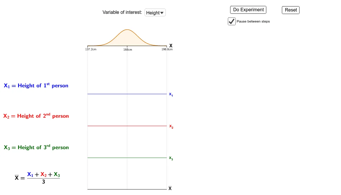
This applet dynamically illustrates the concept of independent identically distributed (i.i.d.) random variables. It demonstrates how multiple random samples are drawn from a chosen distribution, how their empirical distributions approximate the theoretical one, and how sample means behave across experiments. Core mathematical concepts include random variables, independence, identical distribution, sample mean, and the law of large numbers. The construction uses GeoGebra commands such as Sequence, RandomUniform, If, Translate, Segment, and IntegralBetween to generate sample data, plot distribution curves, and animate mean trajectories. Interactive elements include a dropdown menu (distributionDropdown) to switch between distributions and sliders (e.g., dpscale) to adjust precision. Suitable for high school and undergraduate probability and statistics courses, this applet helps learners grasp the meaning of i.i.d. assumptions and the variability of sample statistics.
GeoGebra Commands & Parameters
Sequence(If[distribution ≟ 1, RandomNormal[0.5, 0.13], InverseGamma[α, β, RandomUniform[0, 1]]], i, 1, 1000) → datalist3rawSequence(If[distribution ≟ 1, RandomNormal[0.5, 0.13], InverseGamma[α, β, RandomUniform[0, 1]]], i, 1, 1000) → datalist2rawSequence(If[distribution ≟ 1, RandomNormal[0.5, 0.13], InverseGamma[α, β, RandomUniform[0, 1]]], i, 1, 1000) → datalist1rawZip((xx + yy + zz) / 3, xx, datalist1, yy, datalist2, zz, datalist3) → meanlistrawElement(datalist1, experiment) → x1activeIf(distribution ≟ 1, F1, F2) → FRandomUniform(4.5, F(x1active)) → y1Element(datalist2, experiment) → x2activeRandomUniform(4.5, F(x2active)) → y2Element(datalist3, experiment) → x3activeRandomUniform(4.5, F(x3active)) → y3Element(datalist3, 4) → x43Element(datalist3, 3) → x33Element(datalist3, 2) → x23Element(datalist3, 1) → x13Element(datalist2, 4) → x42Element(datalist2, 3) → x32Element(datalist2, 2) → x22Element(datalist2, 1) → x12Element(datalist1, 4) → x41Element(datalist1, 3) → x31Element(datalist1, 2) → x21Element(datalist1, 1) → x11Element(meanlist, 1) → m1Element(meanlist, 2) → m2If(distribution ≟ 1, ((x - 0.5) / 0.13 * 8) + 168, (x * 100)) → scalefuncIf(distribution ≟ 1, "cm", "k") → unitsElement({x11dp, x21dp, x31dp, x41dp}, experiment) → x1dpactiveElement({x12dp, x22dp, x32dp, x42dp}, experiment) → x2dpactiveElement({x13dp, x23dp, x33dp, x43dp}, experiment) → x3dpactiveElement(meanlist, 3) → m3Element(meanlist, 4) → m4Element({m1dp, m2dp, m3dp, m4dp}, experiment) → mdpactiveTranslate(DotPlot[Take[datalist2, 1, experiment], false, 0.006], (0, 2 + dpscale / 2)) → datalist2_{dp}underlayerTranslate(DotPlot[Take[datalist1, 1, experiment], false, 0.006], (0, 3 + dpscale / 2)) → datalist1_{dp}underlayerTranslate(DotPlot[Take[datalist3, 1, experiment], false, 0.006], (0, 1 + dpscale / 2)) → datalist3_{dp}underlayerSegment((0, 4.5), (1, 4.5)) → aIntegralBetween(4.5, F, 0, 1, false) → cSegment((0, 0), (1, 0)) → maxisIf(distribution ≟ 1, "", "\$") → dollarsTranslate(F, (0, (-1.5 * t51))) → x1FTranslate(F, (0, (-2.5 * t51))) → x2FTranslate(F, (0, (-3.5 * t51))) → x3FIf(distribution ≟ 1, M1, M2) → MSegment((0, 4.5), (0, 4.45)) → tick1Segment((1, 4.5), (1, 4.45)) → tick3Segment((0.5, 4.5), (0.5, 4.45)) → tick2Segment((0, 2.99), (1, 2.99)) → x1axisSegment((0, 1.99), (1, 1.99)) → x2axisSegment((0, 0.99), (1, 0.99)) → x3axisTranslate(DotPlot[Take[meanlist, 1, experiment], false, 0.006], (0, dpscale / 2)) → Mean_{dp}Segment((0, 4.5), (0, 0)) → guideline1Segment((1, 4.5), (1, 0)) → guideline2Segment((0.5, 4.5), (0.5, 0)) → guideline3
AI Drawing Prompt Reference
Create a probability statistics illustration showing independent identically distributed random variables. Display three horizontal axes, each representing a sample of 1000 points drawn from a chosen distribution (normal or inverse gamma, switchable via a dropdown). On each axis, show a dot plot of sampled points and overlay the theoretical distribution curve. Use vertical segments to connect corresponding sample points across the three axes, representing one experiment's three independent observations. Show a trajectory of sample means across experiments, converging to the theoretical mean. Include axis ticks, a baseline, and a slider to adjust display precision. Label units (cm or k) appropriately. The layout should clearly demonstrate how sample statistics vary and approximate the theoretical distribution.
The prompt above was compiled from the original drawing commands and is for reference only.