
Visualizing Confidence Intervals
Loading the math board and drawing, please wait…
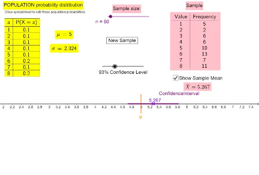
This example dynamically generates samples and displays their confidence intervals to visually demonstrate the concept of confidence intervals. Key math concepts include confidence intervals, sample mean, and normal distribution. It uses commands like Sum, Segment, Sequence, Frequency, FrequencyTable, mean, InverseNormal, LaTeX, Midpoint, TableText in GeoGebra. Suitable for high school students and beginners in probability statistics.
GeoGebra Commands & Parameters
Sum(B2:I2) → J2Sum(B3:I3) → J3Segment((μ, -1), (μ, 1)) → fSequence(RandomDiscrete[xValues, probabilities], k, 1, n) → RandomSampleFrequency(RandomSample) → FrequenciesfromRandomSampleFrequencyTable(RandomSample) → text3mean(RandomSample) → SampleMeanInverseNormal(0, 1, (1 + p_1) / 2) → kSum(B6:I6) → J6LaTeX(μ, true, true) → text7LaTeX(σ, true, true) → text8Segment((LowerBound, 0), (UpperBound, 0)) → ConfidenceIntervalMidpoint(ConfidenceInterval) → BTableText({{A1, B1, C1, D1, E1, F1, G1, H1, I1}, {A2, B2, C2, D2, E2, F2, G2, H2, I2}}, "vc|_cllllllll") → text1