
Visualizing Algebraic Terms: Rotating Cone and Cylinder
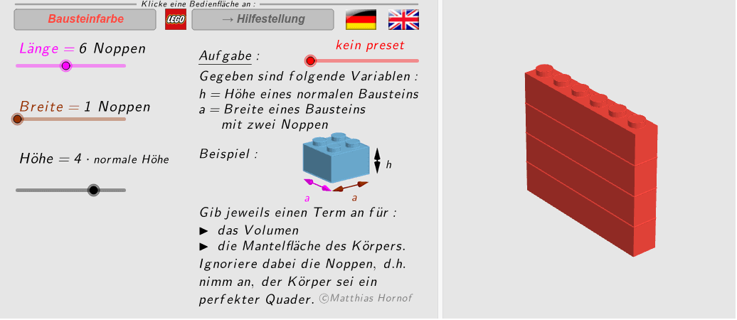
Loading the math board and drawing, please wait…
① This example dynamically demonstrates how algebraic terms (Terme) relate to geometric solids by rotating a cone and a cylinder, making abstract expressions tangible. ② Core mathematical concepts include algebraic expressions, geometric mean, solids of revolution, volume and surface area of cones and cylinders, and ratios. ③ Construction highlights: using GeoGebra commands such as Circle, Cylinder, Polygon, Midpoint, Vector, Sequence, Segment, and SelectedElement, the model builds multiple auxiliary objects (e.g., r_2, h, c, v_z, v_y, v_x, b, a, O, Lh, A_1) to create rotating solids with sliders and sequences, and annotates key dimensions via midpoints, vectors, and segments. ④ Suitable for middle and high school mathematics, especially in courses linking algebra and geometry, to help students grasp the geometric meaning of algebraic terms, enhance spatial reasoning, and support mathematical modeling.
GeoGebra Commands & Parameters
Circle(O, r_1, zAxis) → c_1Cylinder(c_1, h_1) → a_1, d, fPolygon(A_1, A_2, A_3, A_4) → F_0, a_2, a_3, a_4, a_5Polygon(A_1, A_2, B_2, B_1) → F_1, a_6, a_7, b_2, b_3Polygon(A_2, A_3, B_3, B_2) → F_2, a_8, a_9, b_4, b_5Polygon(A_3, A_4, B_4, B_3) → F_3, a_{10}, a_{11}, b_6, b_7Polygon(A_4, A_1, B_1, B_4) → F_4, a_{12}, a_{13}, b_8, b_9Midpoint(B_4, B_1) → B_5Vector(B_5 + (0, 0, -0.3), B_1 + (0, 0, -0.3)) → v_{a1}Vector(B_5 + (0, 0, -0.3), B_4 + (0, 0, -0.3)) → v_{a2}Midpoint(A_1, B_1) → C_1Vector(C_1 + (0.2, 0.2, 0), A_1 + (0.2, 0.2, 0)) → v_{h1}Vector(C_1 + (0.2, 0.2, 0), B_1 + (0.2, 0.2, 0)) → v_{h2}Polygon(A_1 - (h / 3 * v_z), A_2 - (h / 3 * v_z), A_3 - (h / 3 * v_z), A_4 - (h / 3 * v_z)) → U_1, g, i, j, kSequence(Polygon[A_1 + (i * (0, 0, (-h))), A_2 + (i * (0, 0, (-h))), A_3 + (i * (0, 0, (-h))), A_4 + (i * (0, 0, (-h)))], i, 1, c - 3) → UVector(Midpoint[B_3 + (0, 0, -0.3), B_4 + (0, 0, -0.3)], B_4 + (0, 0, -0.3)) → v_{b1}Vector(Midpoint[B_3 + (0, 0, -0.3), B_4 + (0, 0, -0.3)], B_3 + (0, 0, -0.3)) → v_{b2}Circle(O + (0, 0, z(B_1)), r_2, zAxis) → c_2Cylinder(c_2, Min[0.92, (Element[Lh, c] * h) - 0.08] - 0.05) → zyl_3, p, lPolygon(B_1, B_2, B_3, B_4) → F_5, b_1, b_{10}, b_{11}, b_{12}Segment(Pos_2, Pos_2 + (11.3, 0)) → mSelectedElement(Lcol) → elSequence(Sequence[Sequence[Translate[zyl_3, Vector[(i * v_x) + (j * v_y) + ((k * v_z) * h)]], i, ((-a)) / 2 + 1, a / 2 - 1], j, ((-b)) / 2 + 1, b / 2 - 1], k, 0, c - 3) → untSequence(Sequence[Sequence[Translate[a_1, Vector[((i - a / 2 - 1 / 2) * v_x) + ((j - b / 2 - 1 / 2) * v_y) + (((0.5 * Element[Lh, c]) * h) * v_z) - ((k * v_z) * h)]], i, 1, a], j, 1, b], k, 0, Max[c - 3, 0]) → e
AI Drawing Prompt Reference
Create a dynamic visualization showing the relationship between algebraic terms and geometric solids by rotating a cone and a cylinder. Construct the cone and cylinder using polygons, then use sliders and sequences to control their dimensions. Annotate key measurements and create rotating solids. The final image should include the rotating cone and cylinder, along with auxiliary objects and sequences, demonstrating volume and surface area calculations.
The prompt above was compiled from the original drawing commands and is for reference only.