
Boxplot of Time Series
Loading the math board and drawing, please wait…
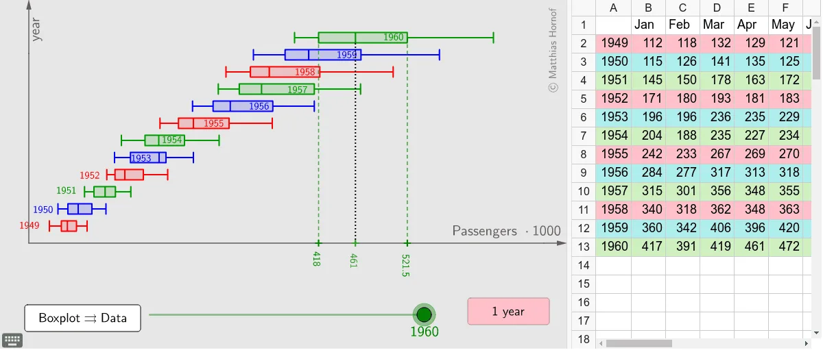
This example demonstrates the boxplot analysis of time series data. A boxplot is a statistical chart that shows the distribution of data, including the median, quartiles, and outliers. The core mathematical concepts involved include statistics such as the median, quartiles, and construction of boxplots. Using GeoGebra commands like Flatten, Sequence, PolyLine, and BoxPlot, the distribution characteristics of the data can be visually presented. Suitable for high school and above students to learn data statistics and analysis.
GeoGebra Commands & Parameters
Flatten({l1, l2, l3, l4, l5, l6, l7, l8, l9, l10, l11, l12}) → LSequence(Segment[((1.2 * i) + 0.6, 0), ((1.2 * i) + 0.6, -20)], i, 0, 11) → l14PolyLine(Sequence[((sclx * (i - 1)), (scly * Element[L, i])), i, 1, 12]) → lp1PolyLine(Sequence[((sclx * (i - 1)), (scly * Element[L, i])), i, 24, 36]) → lp3PolyLine(Sequence[((sclx * (i - 1)), (scly * Element[L, i])), i, 12, 24]) → lp2PolyLine(Sequence[((sclx * (i - 1)), (scly * Element[L, i])), i, 36, 48]) → lp4PolyLine(Sequence[((sclx * (i - 1)), (scly * Element[L, i])), i, 48, 60]) → lp5PolyLine(Sequence[((sclx * (i - 1)), (scly * Element[L, i])), i, 60, 72]) → lp6PolyLine(Sequence[((sclx * (i - 1)), (scly * Element[L, i])), i, 72, 84]) → lp7PolyLine(Sequence[((sclx * (i - 1)), (scly * Element[L, i])), i, 96, 108]) → lp9PolyLine(Sequence[((sclx * (i - 1)), (scly * Element[L, i])), i, 108, 120]) → lp10PolyLine(Sequence[((sclx * (i - 1)), (scly * Element[L, i])), i, 120, 132]) → lp11PolyLine(Sequence[((sclx * (i - 1)), (scly * Element[L, i])), i, 132, 144]) → lp12Sequence(50 + (50 * i), i, 0, 11) → LbpyBoxPlot(Element[Lbpy, 1], 15, (sclbx * l1) - bxoff) → a1BoxPlot(Element[Lbpy, 2], 15, (sclbx * l2) - bxoff) → a2BoxPlot(Element[Lbpy, 3], 15, (sclbx * l3) - bxoff) → a3BoxPlot(Element[Lbpy, 4], 15, (sclbx * l4) - bxoff) → a4BoxPlot(Element[Lbpy, 5], 15, (sclbx * l5) - bxoff) → a5BoxPlot(Element[Lbpy, 6], 15, (sclbx * l6) - bxoff) → a6BoxPlot(Element[Lbpy, 7], 15, (sclbx * l7) - bxoff) → a7BoxPlot(Element[Lbpy, 8], 15, (sclbx * l8) - bxoff) → a8BoxPlot(Element[Lbpy, 9], 15, (sclbx * l9) - bxoff) → a9BoxPlot(Element[Lbpy, 10], 15, (sclbx * l10) - bxoff) → a10BoxPlot(Element[Lbpy, 11], 15, (sclbx * l11) - bxoff) → a11BoxPlot(Element[Lbpy, 12], 15, (sclbx * l12) - bxoff) → a12Vector((0, 0), (x(Corner[1, 2]), 0)) → vx2Vector((0, 0), (0, y(Corner[1, 4]))) → vy2Point(vy2) → ASegment(Qu, Qu + (0, Element[Lbpy, m])) → squSegment(Qo, Qo + (0, Element[Lbpy, m])) → sqoQ1(Element[LNR, m]) → quQ3(Element[LNR, m]) → qoSegment(Md1, Md1 + (0, Element[Lbpy, 1] - 15)) → sm1Segment(Md2, Md2 + (0, Element[Lbpy, 2] - 15)) → sm2Segment(Md3, Md3 + (0, Element[Lbpy, 3] - 15)) → sm3Segment(Md4, Md4 + (0, Element[Lbpy, 4] - 15)) → sm4Segment(Md5, Md5 + (0, Element[Lbpy, 5] - 15)) → sm5Segment(Md6, Md6 + (0, Element[Lbpy, 6] - 15)) → sm6Segment(Md7, Md7 + (0, Element[Lbpy, 7] - 15)) → sm7Segment(Md8, Md8 + (0, Element[Lbpy, 8] - 15)) → sm8Segment(Md9, Md9 + (0, Element[Lbpy, 9] - 15)) → sm9Segment(Md10, Md10 + (0, Element[Lbpy, 10] - 15)) → sm10Segment(Md11, Md11 + (0, Element[Lbpy, 11] - 15)) → sm11Segment(Md12, Md12 + (0, Element[Lbpy, 12] - 15)) → sm12Point(vx2) → CPolyLine(Sequence[((sclx * (i - 1)), (scly * Element[L, i])), i, 84, 96]) → lp8
AI Drawing Prompt Reference
Draw a boxplot of time series data, consisting of 12 boxplots, each representing the data distribution of a time period. First, draw a line graph of 12 data points, then draw 12 boxplots, each containing the median, quartiles, and outliers. Finally, draw the x-axis and y-axis.
The prompt above was compiled from the original drawing commands and is for reference only.