Unit Circle Trigonometric Lines and Graphs of Six Functions

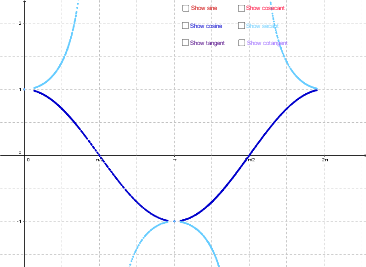
① This GeoGebra example dynamically demonstrates the geometric construction of trigonometric line segments (sine, cosine, tangent, cotangent, secant, cosecant) on the unit circle, while simultaneously plotting the graphs of the six corresponding trigonometric functions, visually linking the unit circle geometry to function graphs. ② Core mathematical concepts include the unit circle definition of trigonometric functions, directed line segments, periodicity, and the dynamic relationship between angle changes and function values. ③ Construction highlights: using GeoGebra commands such as Intersect, Point, CircleArc, Segment, Angle, and OrthogonalLine, the example builds a unit circle c, a movable point A, radius r, angle α, and generates the trigonometric line objects (sine, cosine, tangent, secant, cosecant, cotangent), along with function graphs f, g, h, j, etc., and text labels (text1–text6) for function names. ④ Suitable for high school or pre-university students learning trigonometric definitions and graphs, and useful for classroom demonstrations or self-exploration of how angle changes affect function values, bridging geometric and algebraic representations.