
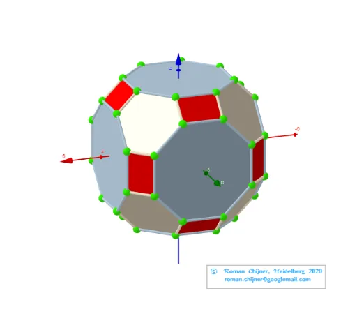
Truncated Cuboctahedron: Vertex Average Distance vs. Truncation Parameter
Loading the math board and drawing, please wait…
This example demonstrates the dependence of the average distance between vertices of a truncated cuboctahedron on its truncation parameter, highlighting extreme distribution patterns. Key mathematical concepts include polyhedron geometry, parameterization, average distance calculation, and optimization problems. GeoGebra commands like Join, Unique, Length, Sphere, Zip, Ray, and others are used to construct the model dynamically, showing how parameter changes affect vertex distances. Suitable for high school students and math enthusiasts exploring polyhedral properties and parametric geometry.
GeoGebra Commands & Parameters
Join(Zip[lP0(x(a)) + ((lP0(y(a)) - lP0(x(a))) * {t, 1 - t}), a, segN]) → lVVUnique(lVV) → lP'Length(lP') → nLength(lVV(1)) → R2Sphere(O, R1) → sp1Sphere(O, R2) → sp2Zip(Polygon[a], a, v_poly06) → poly06Zip(Segment[lP0(x(a)), lP0(y(a))], a, segN1) → seg1Zip(Segment[lP0(x(a)), lP0(y(a))], a, segN2) → seg2Zip(Polygon[a], a, v_poly04) → poly04Zip(Polygon[a], a, v_poly08) → poly08Ray(B, AA) → hUnicodeToLetter(34) → u34Text("" + p3) → txt_pSum(Flatten[Sequence[Append[Sequence[Element[txt_p, i], i, m1(k), m2(k)], " "], k, 1, 5]]) → txtUm1Zip(Segment[lVV(x(a)), lVV(y(a))], a, segNΔ4) → segΔ4Zip(Segment[lVV(x(a)), lVV(y(a))], a, segNΔ6) → segΔ6Zip(Segment[lVV(x(a)), lVV(y(a))], a, segNΔ8) → segΔ8TableText(Append["\;\;\; \fgcolor{red}{4-gons}", segΔ4], Append["\;\;\; \fgcolor{#FFBF00}{6-gons}", segΔ6], Append["\;\;\; \fgcolor{#5D8AA8}{8-gons}", segΔ8], "v") → text3a