
Trapezium Rule Demonstration by Vivax Solutions
Loading the math board and drawing, please wait…
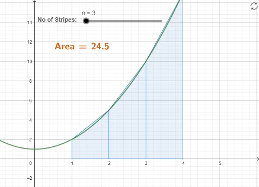
This example demonstrates the Trapezium Rule for numerical integration, visually showing how adjusting the number of intervals and the function graph approximates the true integral. Core mathematical concepts include numerical integration, trapezoidal approximation, function graphing, and interval partitioning. It uses GeoGebra commands like `TrapezoidalSum` for calculating the trapezoidal sum, `LaTeX` for text rendering, and objects such as `f` (function), `n` (number of intervals), `a` (interval), `Area` (area calculation), and `text1`, `text2` for visualization. Suitable for high school students and above learning numerical integration methods in calculus, or as a mathematical demonstration tool.
GeoGebra Commands & Parameters
TrapezoidalSum(f, 1, 4, n) → aLaTeX(Area, true, true) → text1
AI Drawing Prompt Reference
Draw a graphical demonstration of the trapezoidal rule for numerical integration. The graph should include a function curve, interval division markers, and the area calculated by the trapezoidal approximation. The approximate value should gradually approach the true integral as the number of intervals increases. The graph should clearly show the relationship between the function, intervals, and area to help understand the concept of numerical integration.
The prompt above was compiled from the original drawing commands and is for reference only.