
Traffic Speed 2
Loading the math board and drawing, please wait…
In collections
Traffic
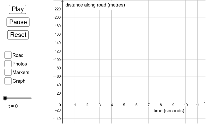
This example demonstrates the changes in traffic speed. Key mathematical concepts include the relationship between speed, acceleration, and time. Using GeoGebra commands such as Sequence and Segment, the speed curve can be dynamically displayed. Suitable for high school physics and mathematics education.
GeoGebra Commands & Parameters
Sequence((n, g(n)), n, 0, t_1) → list2Segment((-1.9, 0), (-1.1, 0)) → road_0Sequence(i - 0.4 < x < i + 0.4, i, 0, t_1) → photo_{road}Sequence(x = i - 0.4, i, 0, t_1) → left_{road}Sequence(x = i + 0.4, i, 0, t_1) → right_{road}Sequence(x = i, i, 0, t_1) → mid_{road}Sequence(Translate[car_p, Vector[(0, g(0)), (i - g_y(i), g(i))]], i, 0, t_1) → photo_rSegment((-1.9, 200), (-1.1, 200)) → road_{200}