
Three Forms of Decimal
Loading the math board and drawing, please wait…
In collections
Decimals
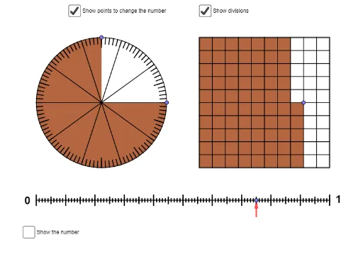
This example demonstrates the three forms of decimals: finite decimals, infinite repeating decimals, and infinite non-repeating decimals. Key mathematical concepts include sequences, circles, and coordinate geometry. Using GeoGebra commands such as Circle, Sequence, and Point, the transition process of decimals can be dynamically displayed. Suitable for students at the junior high school level and above to learn about decimal concepts.
GeoGebra Commands & Parameters
Circle((0, 0), 1) → cSequence(Point[{cos(((i * 2) * π / 10)), sin(((i * 2) * π / 10))}], i, 0, 9) → list1Zip(Segment[(0, 0), A], A, list1) → list2Sequence(Point[{cos(((i * 2) * π / 100)), sin(((i * 2) * π / 100))}], i, 0, 99) → list3Sequence(Point[{(0.9 * cos(((i * 2) * π / 100))), (0.9 * sin(((i * 2) * π / 100)))}], i, 0, 99) → list4Zip(Segment[A, B], A, list3, B, list4) → list5Point(list3) → APoint(list3) → BSector(c, A, B) → dSequence(Point[{cos(((i * 2) * π / 10) + π / 10), sin(((i * 2) * π / 10) + π / 10)}], i, 0, 9) → list6Zip(Segment[A, (0.85 * A)], A, list6) → list7Polygon((1.5, -1), (3.5, -1), 4) → squareOutlineRemove(Flatten[Sequence[Sequence[Point[{i, j}], j, -1, 1, 0.2], i, 1.7, 3.5, 0.2]], {(3.5, 1)}) → squarePointsMod(100 - (IndexOf[A, list3] - IndexOf[B, list3]), 100) → circleSizePoint(squarePoints) → CVertex(squareOutline) → D, E, F, GSegment(G, F) → fSegment(F, E) → gSegment(E, D) → hSegment(D, G) → iOrthogonalLine(C, f) → jOrthogonalLine(C, g) → kIntersect(j, f) → HIntersect(k, i) → IIntersect(j, h) → JOrthogonalLine(K, k) → lIntersect(k, l) → LFlatten(Sequence[Sequence[Point[{i, j}], j, -1, 0.8, 0.2], i, 1.7, 3.5, 0.2]) → backupSquarePointsIntersect(l, h) → MPolygon(D, G, K, L, C, J) → poly1, d_1, g_1, k_1, l_1, c_1, j_1Sequence(Point[{i, -1.5}], i, -1, 3.5 - 0.045, 0.045) → linePointsPoint(linePoints) → NSegment((-1, -1.5), (3.5, -1.5)) → mSequence(Segment[(i, -1.525), (i, -1.475)], i, -1, 3.5, 0.045) → L_2Vector(N - (0, 0.25), N) → uSequence(Segment[(i, -1.55), (i, -1.45)], i, -1 + 0.45 / 2, 3.5, 0.45) → L_3Sequence(Segment[(i, -1.58), (i, -1.42)], i, -1, 3.5, 0.45) → L_1Sequence(Segment[(1.5, j), (3.5, j)], j, -0.8, 0.8, 0.2) → L_4Sequence(Segment[(i, -1), (i, 1)], i, 1.7, 3.3, 0.2) → L_5TableText({If[n, FractionText[circleSize / 100], (((("\frac{" * circleSize) * "}{") * 100) * "}")], circleSize / 100, circleSize + "%"}) → text3
AI Drawing Prompt Reference
Draw a unit circle centered at the origin with ten equally spaced points on its circumference, and connect each point to the center with a radius segment. On the same circle, place one hundred densely spaced points, and on a slightly smaller concentric circle, place one hundred corresponding points; connect each outer point to its inner counterpart with a thin radial line. Select two adjacent points on the outer circle and highlight the arc between them. To the right, draw a square grid region with a uniform lattice of points inside, bounded by a square outline. Place a movable point within the grid, drop perpendiculars from it to each side of the square, and construct the polygon formed by these perpendiculars and the square's sides. Below the figure, draw a horizontal number line with tick marks and an arrow, and display a text label showing a fraction, its decimal, and its percentage.
The prompt above was compiled from the original drawing commands and is for reference only.