
The Effect of Extremes: IM Algebra 1 Unit 1 Lesson 10
Loading the math board and drawing, please wait…
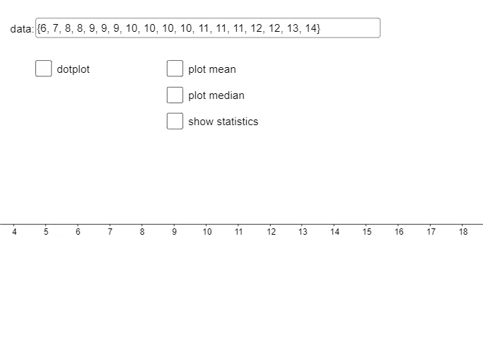
This GeoGebra example demonstrates how adding extreme values (very large or very small) to a dataset affects key statistics such as mean, median, quartiles, and the resulting dot plot, histogram, and box plot. Core mathematical concepts include descriptive statistics: measures of central tendency (mean, median), spread (interquartile range, mean absolute deviation), and the robustness of statistics to outliers. Construction highlights: using GeoGebra commands like Textfield for data input, Min, Max, Sequence, mean, Median, Q1, Q3 for calculations, and Zip, DotPlot, Histogram, BoxPlot for visualizations. Sliders or input boxes allow dynamic adjustment of extreme values. Suitable for upper middle school or high school algebra courses, this interactive lesson helps students intuitively grasp how outliers distort statistical summaries and supports data analysis and critical thinking skills.
GeoGebra Commands & Parameters
Textfield(data) → InputBox1_1Min(data) → mndMax(data) → mxdSequence(hmn + (i * spc), i, 0, hn) → list1Textfield(hmn) → InputBox2_1Textfield(hmx) → InputBox3_1Textfield(spc) → InputBox4_1mean(data) → avgMedian(data) → mdnQ1(data) → dq1Q3(data) → dq3Zip(abs(z - avg), z, data) → list2mean(list2) → madDotPlot(data) → list3Textfield(mxy) → InputBox5_1Histogram(list1, data, false) → cMax(Frequency[data]) → htBoxPlot(1, 0.5, data) → a
AI Drawing Prompt Reference
Create a graph showing the impact of extreme values on a dataset, including input boxes to adjust the data range and spacing, calculate and display the minimum, maximum, mean, median, quartiles, and mean absolute deviation of the dataset, generate a dot plot, histogram, and box plot, and dynamically adjust the input boxes to observe how extreme values change the statistical summary.
The prompt above was compiled from the original drawing commands and is for reference only.