
Surface Area of a Right Cone
Loading the math board and drawing, please wait…
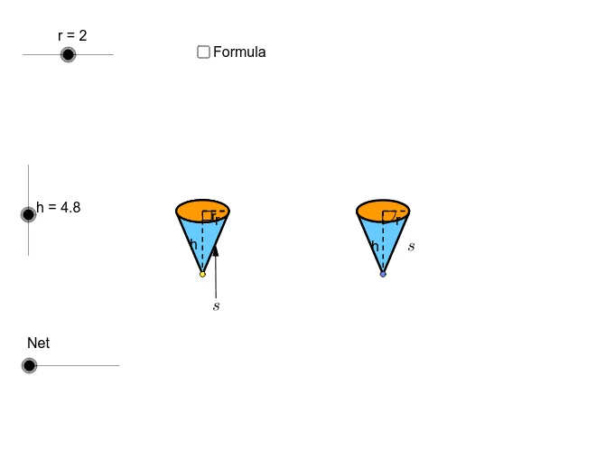
This example demonstrates the calculation of the surface area of a right cone. It involves core mathematical concepts such as the base radius, slant height, and surface area formula. The construction uses GeoGebra commands and objects like Point, Circle, Intersect, Vector, Translate, Rotate, and Polygon to build the cone and compute its surface area, making it suitable for high school students learning solid geometry and surface area calculations.
GeoGebra Commands & Parameters
Point(xAxis) → ACircle(A, r) → cIntersect(c, xAxis) → B, CEllipse(E, D, C) → eIntersect(xAxis, yAxis) → FVector(F, G) → uTranslate(B, Vector[(u * h)]) → B'_1Translate(C, Vector[(u * h)]) → C'_1Translate(A, Vector[(u * h)]) → A'_1Translate(e, Vector[(u * h)]) → e'_1Arc(e'_1, C'_1, B'_1) → p_5Arc(e'_1, B'_1, C'_1) → qSegment(A'_1, A) → h_6Segment(A'_1, C'_1) → pAngle(A, A'_1, C'_1) → αLine(A, A'_1) → jIntersect(e'_1, j) → H, ICircle(I, r) → tIntersect(t, j, 2) → KCircle(K, I) → d_1Intersect(d_1, j, 2) → NVector(H, N) → vTranslate(H, Vector[(v * n)]) → H'_1Translate(D, Vector[(u * h)]) → D'Translate(E, Vector[(u * h)]) → E'Line(B, B'_1) → lLine(C, C'_1) → mIntersect(d_1, l, 1) → PIntersect(d_1, m, 1) → QVector(B'_1, P) → zVector(C'_1, Q) → u_1Translate(B'_1, Vector[(z * n)]) → B''Translate(C'_1, Vector[(u_1 * n)]) → C''Midpoint(B'_1, A'_1) → RMidpoint(B, A) → SLine(R, S) → a_1Intersect(q, a_1) → T,Intersect(d_1, a_1, 1) → UVector(T, U) → v_1Translate(T, Vector[(v_1 * n)]) → T'If(n ≟ 0.01, B'_1, If[n < 1, B'', P]) → B_1If(n ≟ 0.01, T, If[n < 1, T', U]) → D_1If(n ≟ 0.01, H, If[n < 1, H'_1, N]) → E_1If(n ≟ 0.01, C'_1, If[n < 1, C'', Q]) → F_1Conic(B_1, D_1, E_1, F_1, I) → g_1Conic(I, B_1, D_1, E_1, F_1) → h_1OrthogonalLine(I, j) → l_1OrthogonalLine(H, j) → b_2Intersect(m, l_1) → H_2Midpoint(H_2, C'_1) → I_2OrthogonalLine(C'_1, m) → i_2Segment(K, F_1) → m_4Translate(e, Vector[(u * h)]) → e'Tangent(A, e'_1) → a, bIntersect(e', b) → J, G_2Intersect(e', a) → L, R_2Segment(A, J) → fSegment(A, L) → gCircle(I, sqrt(h^(2) + r^(2))) → kIntersect(k, j, 1) → MCircle(M, sqrt(h^(2) + r^(2))) → sSegment(M, I) → iRotate(I, γ, M) → I'_1Rotate(I, (-γ), M) → I'_2OrthogonalLine(I'_2, i_2) → b_1Intersect(b_2, b_1) → OMidpoint(H, O) → VCircle(V, O) → c_1Vector(O, I'_2) → wCenter(g_1) → WSegment(W, F_1) → e_1Vector(H, A) → w_1Translate(H, Vector[(w_1 * (n - 1))]) → H'If(n < 1, H, If[n < 2, H', A]) → ZSegment(H, Z) → f_1Rotate(I, (-δ), M) → I'Vector(L, I') → z_1Translate(c_1, Vector[(w * (n - 2))]) → k_1Center(k_1) → A_1Intersect(k_1, j) → C_1, Q_1Rotate(C_1, (180° * (n - 2)), A_1) → G_1If(n < 2, H, If[n ≤ 3, G_1, I'_2]) → H_1Mirror(H_1, j) → I_1Translate(L, Vector[(z_1 * (n - 2))]) → L'If(n < 2, L, If[n ≤ 3, L', I']) → J_1Mirror(J_1, j) → K_1Conic(I_1, H_1, J_1, I, K_1) → p_1Vector(A, M) → i_1Translate(A, Vector[(i_1 * (n - 2))]) → A'If(n < 2, A, If[n ≤ 3, A', M]) → L_1Tangent(L_1, p_1) → j_1, m_1Intersect(p_1, m_1, 1) → M_1Intersect(p_1, j_1, 1) → N_1Polygon(L_1, M_1, N_1) → poly1, n_1, l_2, m_2Arc(p_1, N_1, M_1) → q_1Line(L_1, b_2) → r_1Intersect(p_1, r_1, 1) → O_1Intersect(p_1, r_1, 2) → P_1Arc(p_1, P_1, O_1) → s_1Polygon(L_1, O_1, I_1) → poly2, i_3, l_3, o_1Polygon(L_1, H_1, P_1) → poly3, p_2, l_4, h_2Arc(p_1, O_1, I_1) → t_1Arc(p_1, H_1, P_1) → c_2Segment(L_1, I_1) → a_2Segment(L_1, H_1) → d_2Arc(p_1, H_1, I_1) → e_2Polygon(I_1, L_1, H_1) → poly4, h_3, i_4, l_5CircleSector(M, I'_2, I'_1) → f_2CircleSector(M, I'_2, I'_1) → g_2Arc(p_1, H_1, I_1) → k_2Segment(M_1, L_1) → j_2Segment(N_1, L_1) → n_2Polygon(I_1, L_1, H_1) → poly5, h_4, i_5, l_6Arc(p_1, H_1, I_1) → q_2Polygon(J, A, L) → poly6, l_7, j_3, a_3Point(xAxis) → R_1OrthogonalLine(R_1, xAxis) → r_2Intersect(i_2, r_2) → S_1Circle(R_1, r) → s_2Intersect(s_2, xAxis) → T_1, U_1OrthogonalLine(T_1, i_2) → t_2OrthogonalLine(V_1, i_2) → b_3OrthogonalLine(W_1, i_2) → c_3Intersect(i_2, t_2) → Z_1Intersect(i_2, b_3) → A_2Intersect(i_2, c_3) → B_2Ellipse(A_2, B_2, Z_1) → d_3Tangent(R_1, d_3) → e_3, f_3Intersect(d_3, f_3, 1) → C_2Intersect(d_3, e_3, 1) → D_2Polygon(C_2, D_2, R_1) → poly7, r_3, c_4, d_4Ellipse(A_2, B_2, Z_1) → g_3OrthogonalLine(U_1, xAxis) → k_3Intersect(g_3, k_3) → E_2, J_2Segment(S_1, E_2) → m_3Segment(S_1, R_1) → n_3Intersect(d_3, m_3, 1) → F_2Midpoint(g) → K_2Midpoint(f_1) → L_2Point(j) → M_2Midpoint(I_1, A') → N_2Midpoint(A', H_1) → O_2Vector(M_2, N_2) → u_2Vector(M_2, O_2) → v_2Line(M_2, r_1) → p_3Point(p_3) → P_2Vector(P_2, K_2) → z_2Vector(P_2, L_2) → u_3Center(g_3) → Q_2Angle(F_2, Q_2, R_1) → εSegment(I_1, H_1) → q_3Intersect(k_2, q_3, 2) → S_2Point(poly7) → T_2
AI Drawing Prompt Reference
Draw a right cone to demonstrate its surface area calculation. Include the base circle, slant height, lateral arc, vertex, and base points. The construction order: first establish a coordinate system and points, draw a circle and an ellipse; then use vector translations to build the cone's vertex, base points, and lateral arc; next calculate angles and line segments; finally draw the cone's lateral surface and perpendicular lines. Key objects include the base radius, slant height, and surface area formula.
The prompt above was compiled from the original drawing commands and is for reference only.