
Surface Area: Introduction - Rectangular Prism Net and Calculation
Loading the math board and drawing, please wait…
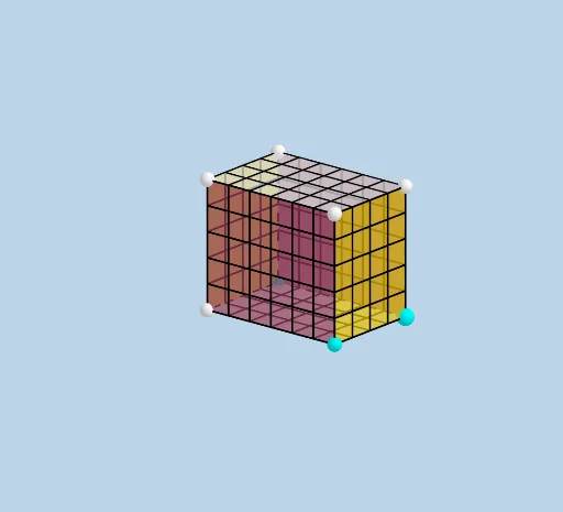
This GeoGebra example demonstrates the concept of surface area by unfolding a rectangular prism into its net, allowing learners to visualize how the total surface area is the sum of the areas of all faces. It bridges 3D solid geometry with 2D representations, making the calculation intuitive. Core mathematical concepts include surface area of prisms, nets, the Pythagorean theorem (for computing diagonal lengths), and indefinite integrals (as a conceptual link to accumulation). The construction uses GeoGebra commands such as Ray, Prism, Net, Sequence, Translate, Vector, and Mirror to build the prism and its six faces (e.g., faceADBE, faceAECF, faceADGF, faceBDGH, faceBECH, faceCFGH), with dynamic elements like sliders to control the unfolding. Suitable for middle school to high school students learning solid geometry, and for teachers demonstrating spatial reasoning and area calculation in class.
GeoGebra Commands & Parameters
Ray((0, 0, 0), (1, 0, 0)) → fRay((0, 0, 0), (0, 1, 0)) → gRay((0, 0, 0), (0, 0, 1)) → hPrism(E, A, D, B, C) → d, F, edgeAE, edgeAD, edgeBD, edgeBE, edgeCE, edgeAF, edgeDG, edgeBH, edgeCF, edgeFG, G, edgeGH, edgeCH, H, faceADBE, faceAECF, faceADGF, faceBDGH, faceBECH, faceCFGHNet(d, openclose) → i, I, R, S, T, U, V, faceIJKL, faceIJNM, faceJKPO, faceKLRQ, faceILST, J, faceMNUV, edgeIJ, edgeJK, edgeKL, edgeIL, edgeIM, edgeMN, edgeJN, edgeJO, edgeOP, K, edgeKP, edgeKQ, edgeQR, edgeLR, edgeLS, edgeST, edgeIT, edgeNU, edgeUV, edgeMV, L, M, N, O, P, QSequence(Segment[(i, 0, 0), (i, WIDTH, 0)], i, 1, LENGTH - 1, 1) → L_1Translate(L_1, Vector[A, F]) → L_2Sequence(Segment[(0, i + 1, 0), (LENGTH, i + 1, 0)], i, 0, WIDTH - 2) → L_3Translate(L_3, Vector[A, F]) → L_4Vector(M, V) → uSequence((x(M) + i, y(M), z(M)), i, 1, LENGTH - 1, 1) → L_5Translate(L_5, u) → L_6Sequence(Segment[Element[L_5, i], Element[L_6, i]], i, 1, LENGTH - 1) → L_7Sequence((x(M), y(M) + (i * y(u) / WIDTH), z(M) + (i * z(u) / WIDTH)), i, 1, WIDTH - 1, 1) → L_8Vector(V, U) → vTranslate(L_8, v) → L_9Sequence(Segment[Element[L_8, i], Element[L_9, i]], i, 1, WIDTH - 1) → L_{10}Vector(A, O) → wSequence((x(A) + (i * x(w) / HEIGHT), y(A), z(A) + (i * z(w) / HEIGHT)), i, 1, HEIGHT - 1, 1) → L_{11}Vector(O, P) → lTranslate(L_{11}, l) → L_{12}Sequence(Segment[Element[L_{11}, i], Element[L_{12}, i]], i, 1, HEIGHT - 1) → L_{13}Sequence((x(O), y(O) + (i * y(l) / WIDTH), z(O) + (i * z(l) / WIDTH)), i, 1, WIDTH - 1, 1) → L_{14}Translate(L_{14}, Vector[(-w)]) → L_{15}Sequence(Segment[Element[L_{14}, i], Element[L_{15}, i]], i, 1, WIDTH - 1) → L_{16}Mirror(L_{13}, k) → L_{17}Mirror(L_{16}, k) → L_{18}Vector(D, Q) → mSequence((x(B) + (i * x(v) / LENGTH), y(B), z(B)), i, 1, LENGTH - 1, 1) → L_{19}Translate(L_{19}, m) → L_{20}Sequence(Segment[Element[L_{19}, i], Element[L_{20}, i]], i, 1, LENGTH - 1) → L_{21}Sequence((x(B), y(B) + (i * y(m) / HEIGHT), z(B) + (i * z(M) / HEIGHT)), i, 1, HEIGHT - 1, 1) → L_{22}Translate(L_{22}, v) → L_{23}Sequence(Segment[Element[L_{22}, i], Element[L_{23}, i]], i, 1, HEIGHT - 1) → L_{24}Mirror(L_{21}, n) → L_{25}Mirror(L_{24}, n) → L_{26}
AI Drawing Prompt Reference
Draw a rectangular prism and its net. Start with three coordinate axes in 3D space, then construct a rectangular prism with six labeled faces. Use a slider to unfold the prism into a flat net of six connected faces. Add grid lines on each face of the net to help calculate areas. Include vectors and segments to show translations and reflections during the unfolding process. The final image should clearly show the relationship between the 3D solid and its 2D net, making surface area calculation intuitive.
The prompt above was compiled from the original drawing commands and is for reference only.