
Static Visualization of Binomial Distribution PDF
Loading the math board and drawing, please wait…
In collections
UNSW MATH1131/1231 Algebra material
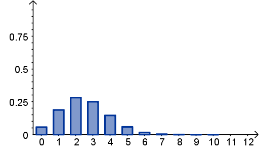
This GeoGebra example presents a static visualization of the binomial distribution, focusing on its probability mass function and cumulative distribution function. It demonstrates how discrete probability values change with the success probability p, the failure probability q, and the number of trials n. The construction uses the Sequence command to generate discrete values, while objects such as d, p, q, n, f, F, Plotf, q_1, q_2, q_3, and PlotF define parameters, build the probability and cumulative functions, plot the corresponding graphs, and mark key probability or quantile points. It is suitable for high school mathematics, introductory probability and statistics courses, teacher demonstrations, and student exploration of binomial distribution shape, spread, and skewness.
GeoGebra Commands & Parameters
Sequence(((n! / i! / (n - i)! * p^(i)) * q^(n - i)), i, 0, n) → fSequence(Sum[Sequence[((n! / i! / (n - i)! * p^(i)) * q^(n - i)), i, 0, k]], k, 0, n) → FSequence(Polygon[(i - d, 0), (i + d, 0), (i + d, Element[f, i + 1]), (i - d, Element[f, i + 1])], i, 0, n, 1) → PlotfSequence(Polygon[(i - d, 0), (i + d, 0), (i + d, Element[F, i + 1]), (i - d, Element[F, i + 1])], i, 0, n, 1) → PlotF
AI Drawing Prompt Reference
Create a static visualization of a binomial distribution. Use parameters for the number of trials, success probability, failure probability, and a small half-width for bars. Compute the probability for each possible number of successes from 0 to the number of trials, and compute the cumulative probabilities by adding these values up to each success count. Draw two sets of rectangular bars along the horizontal axis, centered at each success count. The first set has heights equal to the individual probabilities, representing the probability mass function. The second set has heights equal to the cumulative probabilities, representing the cumulative distribution function. The bars should extend upward from the horizontal axis and show how the discrete distribution changes with the parameters.
The prompt above was compiled from the original drawing commands and is for reference only.