
Spherical Volume: Geometric Construction and Visualization
Loading the math board and drawing, please wait…
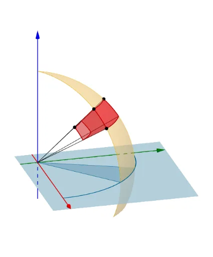
① This GeoGebra example dynamically demonstrates the derivation of the volume of a sphere by parameterizing the spherical surface and constructing internal volume elements. ② Core mathematical concepts include the sphere volume formula, triple integrals, spherical coordinate transformation, parametric surface equations, and the method of infinitesimal elements. ③ Construction highlights: from the summary, commands such as PointIn, If, CurveCartesian, Surface, Intersect, Segment, CircumcircleArc, and CircumcircleSector are used to create points, arcs, sectors, and connecting segments on the sphere. Parameters α and β control the spherical grid, and multiple auxiliary objects (A, B, C, D, etc.) build approximate volume cells inside the sphere. ④ Suitable for upper high school or early university students learning solid geometry and calculus, this example helps visualize the origin of the sphere volume formula and is useful for classroom demonstrations or independent exploration.
GeoGebra Commands & Parameters
PointIn(o) → AIf(x(A) > 0, atan(y(A) / x(A)), atan(y(A) / x(A)) + π) → α_1CurveCartesian((cos(α_1 + t) * sin(β_1)), (sin(α_1 + t) * sin(β_1)), cos(β_1), t, 0, 3.141592653589793) → cPoint(c) → BIf(x(B) > 0, atan(y(B) / x(B)), atan(y(B) / x(B)) + π) → α_2CurveCartesian((cos(α_1) * sin(β_1 + t)), (sin(α_1) * sin(β_1 + t)), cos(β_1 + t), t, 0, π - β_1) → dPoint(d) → CCurveCartesian((cos(α_1 + t) * sin(β_1)), (sin(α_1 + t) * sin(β_1)), cos(β_1), t, 0, Δα) → eSurface((sin(u) * cos(t)), (sin(u) * sin(t)), cos(u), u, β_1, β_2, t, α_1, α_2) → aIntersect(yAxis, zAxis) → ESegment(A, E) → fPoint(f) → FSegment(E, F) → hSegment(F, A) → iSurface(((t * sin(β_1)) * cos(u)), ((t * sin(β_1)) * sin(u)), (t * cos(β_1)), u, α_1, α_2, t, h, 1) → jSurface(((t * sin(β_2)) * cos(u)), ((t * sin(β_2)) * sin(u)), (t * cos(β_2)), u, α_1, α_2, t, h, 1) → kSurface(((t * sin(u)) * cos(α_1)), ((t * sin(u)) * sin(α_1)), (t * cos(u)), u, β_1, β_2, t, h, 1) → lSurface(((t * sin(u)) * cos(α_2)), ((t * sin(u)) * sin(α_2)), (t * cos(u)), u, β_1, β_2, t, h, 1) → mCurveCartesian((cos(α_1 + t) * sin(β_2)), (sin(α_1 + t) * sin(β_2)), cos(β_2), t, 0, Δα) → gCurveCartesian((cos(α_1) * sin(β_1 + t)), (sin(α_1) * sin(β_1 + t)), cos(β_1 + t), t, 0, Δβ) → nCurveCartesian((cos(α_2) * sin(β_1 + t)), (sin(α_2) * sin(β_1 + t)), cos(β_1 + t), t, 0, Δβ) → pSegment(B, B') → qSegment(C, C') → rSegment(D, D') → sCurveCartesian(((h * cos(α_1 + t)) * sin(β_1)), ((h * sin(α_1 + t)) * sin(β_1)), (h * cos(β_1)), t, 0, Δα) → tCurveCartesian(((h * cos(α_1 + t)) * sin(β_2)), ((h * sin(α_1 + t)) * sin(β_2)), (h * cos(β_2)), t, 0, Δα) → uCurveCartesian(((h * cos(α_1)) * sin(β_1 + t)), ((h * sin(α_1)) * sin(β_1 + t)), (h * cos(β_1 + t)), t, 0, Δβ) → vCurveCartesian(((h * cos(α_2)) * sin(β_1 + t)), ((h * sin(α_2)) * sin(β_1 + t)), (h * cos(β_1 + t)), t, 0, Δβ) → wCurveCartesian((cos(α_1 + t) * sin(β_1)), (sin(α_1 + t) * sin(β_1)), cos(β_1), t, 0, 6.283185307179586) → a_1CurveCartesian((cos(α_1 + t) * sin(β_2)), (sin(α_1 + t) * sin(β_2)), cos(β_2), t, 0, 6.28319) → b_1CurveCartesian((cos(α_1) * sin(t)), (sin(α_1) * sin(t)), cos(t), t, 0, 3.141592653589793) → c_1CurveCartesian((cos(α_2) * sin(t)), (sin(α_2) * sin(t)), cos(t), t, 0, 3.141592653589793) → d_1Segment(B, E) → f_1Segment(C, E) → g_1Segment(D, E) → h_1CircumcircleArc(H, C, G) → k_1CircumcircleArc(H, B, G) → p_1Segment(I, E) → i_1Segment(J, E) → j_1Surface((sin(u) * cos(t)), (sin(u) * sin(t)), cos(u), u, 0, β_1, t, α_1, α_2) → m_1Surface(((t * sin(u)) * cos(α_2)), ((t * sin(u)) * sin(α_2)), (t * cos(u)), u, β_1, β_2, t, 0, h) → n_1Surface(((t * sin(u)) * cos(α_2)), ((t * sin(u)) * sin(α_2)), (t * cos(u)), u, 0, β_1, t, 0, 1) → o_1Surface(((t * sin(u)) * cos(α_2)), ((t * sin(u)) * sin(α_2)), (t * cos(u)), u, β_2, 1.5707963267948966, t, 0, 1) → q_1Surface(((t * sin(u)) * cos(α_1)), ((t * sin(u)) * sin(α_1)), (t * cos(u)), u, 0, β_1, t, 0, 1) → r_1Surface(((t * sin(u)) * cos(α_1)), ((t * sin(u)) * sin(α_1)), (t * cos(u)), u, β_2, 1.5708, t, 0, 1) → s_1Surface(((t * sin(u)) * cos(α_1)), ((t * sin(u)) * sin(α_1)), (t * cos(u)), u, β_1, β_2, t, 0, h) → t_1CurveCartesian(cos(t), sin(t), 0, t, 0, 1.5707963267948966) → e_1Surface((sin(u) * cos(t)), (sin(u) * sin(t)), cos(u), u, β_2, 3.141592653589793, t, α_1, α_2) → l_1Surface((t * cos(α_1)), (t * sin(α_1)), u, t, 0, 1, u, -1, 1) → u_1Surface((t * cos(α_2)), (t * sin(α_2)), u, t, 0, 1, u, -1, 1) → v_1CircumcircleSector(I, K, J) → c_2
AI Drawing Prompt Reference
Visualize the derivation of the sphere volume by parameterizing the spherical surface and constructing internal volume elements. The illustration includes multiple auxiliary objects forming approximate volume cells and parameters α and β controlling the spherical grid. Use curves, surfaces, and segments to demonstrate the origin of the sphere volume formula and the method of triple integrals, suitable for classroom demonstrations or student exploration.
The prompt above was compiled from the original drawing commands and is for reference only.