
Space Curves, Velocity and Acceleration
Loading the math board and drawing, please wait…
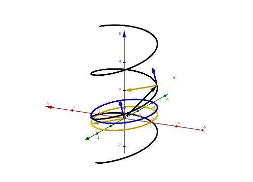
This example demonstrates the plotting of space curves and the visualization of their velocity and acceleration vectors. Key mathematical concepts include space curves, velocity vectors (first derivative), and acceleration vectors (second derivative). It utilizes GeoGebra commands such as CurveCartesian for curve plotting, Vector for vector creation, Derivative for differentiation, Point for point creation, and Translate for translation. Suitable for high school students and teachers studying calculus and analytical geometry.
GeoGebra Commands & Parameters
CurveCartesian(((2 * cos(t)), (3 * sin(t)), t / 2), t, (-4 * π), (4 * π)) → rVector(r(t)) → uDerivative(r) → r'Vector(r'(t)) → wPoint((0, 0), u) → ATranslate(w, A) → vCurveCartesian(r''(x), x, -10, 10) → aVector(a(t)) → sTranslate(s, A) → h
AI Drawing Prompt Reference
Draw a space curve using a parametric equation with a range from -4π to 4π, and display its velocity and acceleration vectors. First, plot the curve, then calculate and draw the velocity vector, placing its tail at the origin. Next, calculate and draw the acceleration vector, also placing its tail at the origin. Finally, plot the trajectories of the velocity and acceleration vectors to show how they change along the curve.
The prompt above was compiled from the original drawing commands and is for reference only.