
Slusher Histogram
Loading the math board and drawing, please wait…
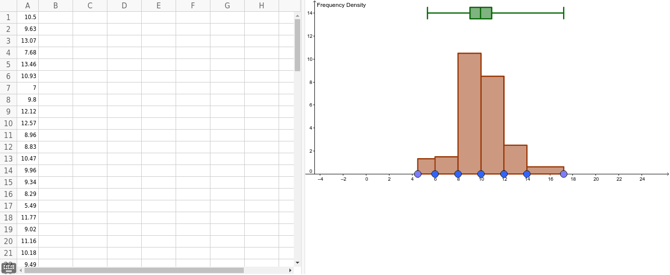
This example demonstrates how to create a Slusher Histogram using GeoGebra, showcasing statistical properties of randomly generated normal distribution data. Core math concepts include histograms, exponential functions, interest calculations, cylinders, differential equations, and box plots. Construction highlights the use of commands like Point, RandomNormal, Ray, Sort, Histogram, and BoxPlot, along with objects such as P_1 to P_30 and A1 to A35. Suitable for high school and above, focusing on data visualization, statistical analysis, and geometric construction integration.
GeoGebra Commands & Parameters
Point(xAxis) → P_1Point(xAxis) → P_4Point(xAxis) → P_2Point(xAxis) → P_5Point(xAxis) → P_3RandomNormal(10, 2) → A1RandomNormal(10, 2) → A2RandomNormal(10, 2) → A3RandomNormal(10, 2) → A4RandomNormal(10, 2) → A5RandomNormal(10, 2) → A6RandomNormal(10, 2) → A7RandomNormal(10, 2) → A8RandomNormal(10, 2) → A9RandomNormal(10, 2) → A10RandomNormal(10, 2) → A11RandomNormal(10, 2) → A12RandomNormal(10, 2) → A13RandomNormal(10, 2) → A14RandomNormal(10, 2) → A15RandomNormal(10, 2) → A16RandomNormal(10, 2) → A17RandomNormal(10, 2) → A18RandomNormal(10, 2) → A19RandomNormal(10, 2) → A20RandomNormal(10, 2) → A21RandomNormal(10, 2) → A22RandomNormal(10, 2) → A23RandomNormal(10, 2) → A24RandomNormal(10, 2) → A25RandomNormal(10, 2) → A26RandomNormal(10, 2) → A27RandomNormal(10, 2) → A28RandomNormal(10, 2) → A29RandomNormal(10, 2) → A30RandomNormal(10, 2) → A31RandomNormal(10, 2) → A32RandomNormal(10, 2) → A33RandomNormal(10, 2) → A34RandomNormal(10, 2) → A35RandomNormal(10, 2) → A36RandomNormal(10, 2) → A37RandomNormal(10, 2) → A38RandomNormal(10, 2) → A39RandomNormal(10, 2) → A40RandomNormal(10, 2) → A41RandomNormal(10, 2) → A42RandomNormal(10, 2) → A43RandomNormal(10, 2) → A45RandomNormal(10, 2) → A46RandomNormal(10, 2) → A47RandomNormal(10, 2) → A48RandomNormal(10, 2) → A49RandomNormal(10, 2) → A50RandomNormal(10, 2) → A44Ray(Left, Left_1) → leftrayRay(Right, Right_1) → rightrayPoint(leftray) → P_0Point(rightray) → P_6Sort(Sequence[x(Element[Points, i + 1]), i, 0, 6]) → BoundariesHistogram(Boundaries, A1:A50) → histogramBoxPlot(14, 0.5, A1:A50) → boxplot
AI Drawing Prompt Reference
Create a slasher histogram to visualize randomly generated normal distribution data. First, create 38 points on the x-axis named P_1 to P_38, then generate 40 sets of random normal distribution data named A1 to A40, and finally use these data to draw the histogram.
The prompt above was compiled from the original drawing commands and is for reference only.