
Slope Field: Differential Equation Visualization
Loading the math board and drawing, please wait…
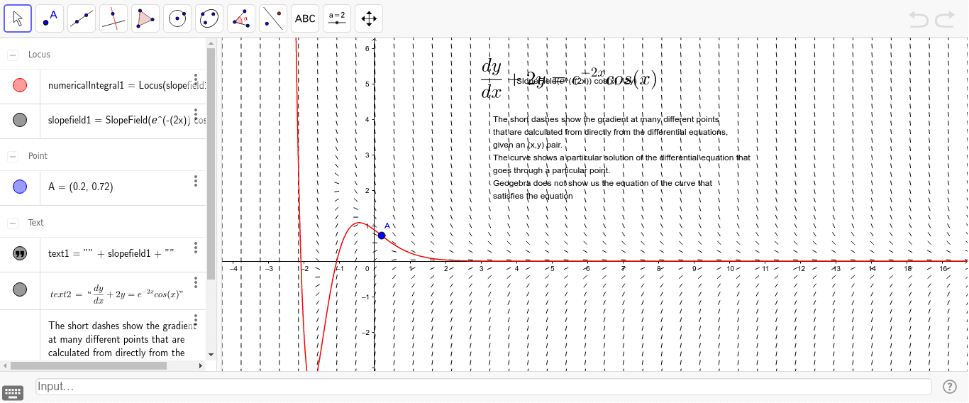
This example demonstrates the slope field of a differential equation, showing the dynamic changes of solution curves. The core mathematical concepts involve differential equations, slope fields, and loci. Construction points include using the SlopeField command, Locus object, numericalIntegral1, etc. GeoGebra commands. Suitable for high school students or college undergraduates for learning differential equations and geometric construction.
GeoGebra Commands & Parameters
SlopeField((ℯ^((-((2 * x)))) * cos(x)) - (2 * y)) → slopefield1Locus(slopefield1, A) → numericalIntegral1
AI Drawing Prompt Reference
Draw the slope field for the differential equation exp(-2x) * cos(x) - 2y. Then, based on this slope field, draw a locus to show the changes in the solution curves of the differential equation.
The prompt above was compiled from the original drawing commands and is for reference only.