
Simple SIR Model
Loading the math board and drawing, please wait…
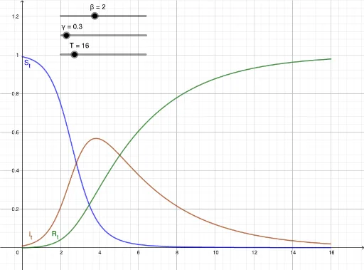
This example demonstrates the dynamic process of the SIR model (Susceptible-Infected-Recovered model). Key math concepts include calculus, differential equations, and probability & statistics. It uses GeoGebra's NSolveODE command to solve differential equations, involving objects like N (total population), β (infection rate), γ (recovery rate), T (time), I_0 (initial infected), S_0 (initial susceptible), R_0 (initial recovered), S', I', R' (rates of change for susceptible, infected, recovered), and S_t, I_t, R_t (populations at time t). Suitable for high school and above learning about epidemiology and differential equations.
GeoGebra Commands & Parameters
NSolveODE({S', I', R'}, 0, {S_0, I_0, R_0}, T) → S_t, I_t, R_t
AI Drawing Prompt Reference
Draw a dynamic diagram of the SIR epidemic model. The horizontal axis represents time, and the vertical axis represents population size. Use three distinct colored curves to show the susceptible, infected, and recovered populations over time. Initially, the susceptible population is near the total population, infected has a small initial value, and recovered starts at zero. As time progresses, the susceptible curve declines, the infected curve rises then falls, and the recovered curve steadily increases. Label key parameters such as total population, infection rate, and recovery rate, and illustrate the rate-of-change relationships described by differential equations. The overall picture shows the classic three-group dynamic balance in epidemiology.
The prompt above was compiled from the original drawing commands and is for reference only.