
Similarity in 1, 2, and 3 Dimensions
Loading the math board and drawing, please wait…
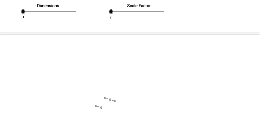
This example dynamically demonstrates similarity transformations in 1D, 2D, and 3D spaces, illustrating core concepts like proportionality, area, volume, rhombus, hyperbola, rational numbers, roots, and cosine functions. It leverages GeoGebra commands such as Polygon, Sequence, Prism, and Segment to construct interactive models. Suitable for high school and advanced learners to explore the nature and calculations of similarity across dimensions.
GeoGebra Commands & Parameters
Polygon(A, B, B + (0, 1, 0), A + (0, 1, 0)) → poly1, a, b, g, hSequence(Segment[(k, 0, 0), (k + 1, 0, 0)], k, 0, d - 1) → list1Sequence((k, 0, 0), k, 0, d) → list2Prism(Polygon[A, B, B + (0, 1, 0), A + (0, 1, 0)], A + (0, 0, 1)) → e, C, edgeBC, edge2, edge3, edge4, edgeCD, edgeDE, edge5, D, E, face1, face3, face4, face2, face5, edge1Segment(A, B) → fSequence(Sequence[Sequence[Cube[(r, s, t), (r, s + 1, t), Point[Circle[(r, s + 1, t), Distance[(r, s, t), (r, s + 1, t)], Segment[(r, s, t), (r, s + 1, t)]]]], r, 1, 10], s, 0, 9], t, 0, 9) → list3Sequence(Sequence[Sequence[Cube[(r, s, t), (r, s + 1, t), Point[Circle[(r, s + 1, t), Distance[(r, s, t), (r, s + 1, t)], Segment[(r, s, t), (r, s + 1, t)]]]], r, 1, 2], s, 0, 1], t, 0, 1) → list5Sequence(Sequence[Polygon[(i, j, 0), (i + 1, j, 0), 4, xOyPlane], i, 0, 1], j, 0, 1) → list4Sequence(Sequence[Polygon[(i, j, 0), (i + 1, j, 0), 4, xOyPlane], i, 0, 9], j, 0, 9) → list6