Section 3.10: Linear Approximation

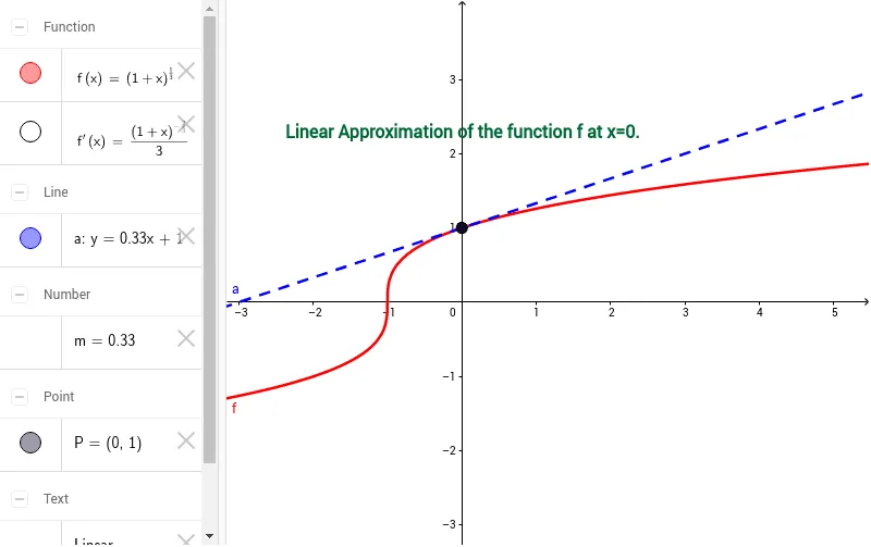
This GeoGebra example demonstrates the concept of linear approximation, also known as tangent line approximation, by showing how the tangent line at a point on a curve can be used to estimate function values near that point. The core mathematical concept is the derivative and the equation of the tangent line. The construction involves defining a function f, computing its derivative f', setting a point a, constructing the tangent line m at that point, marking the point P on the curve, and adding a text1 to display the linear approximation formula. This example is suitable for introductory calculus courses or advanced high school mathematics, helping students visualize the relationship between the derivative and local linearity, and understand how differentials are used for approximation.