Section 14.1 - Level Curves and Surfaces

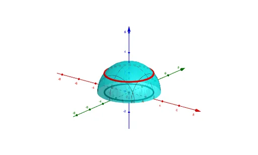
This GeoGebra example visualizes level curves and level surfaces for multivariable functions, showing how sets of points with constant function values appear as curves in the plane or surfaces in space. It demonstrates the core calculus concept of level sets, where varying the parameter k produces different horizontal slices of the function graph, revealing the relationship between contour spacing and the function's rate of change. The construction uses the CurveCartesian command with parameters k, b, c, a, and d, where k acts as a slider controlling the contour height, while other parameters adjust the function form or domain. This is ideal for Calculus III instruction on multivariable functions, partial derivatives, and gradient geometry, as well as for student exploration of how contour density indicates steepness. Suitable for university-level mathematics courses and interactive learning.