
Scatter Plot and Line of Best Fit with Residuals
Loading the math board and drawing, please wait…
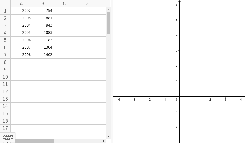
This GeoGebra example demonstrates how to create a scatter plot from discrete data points and automatically fit a line of best fit (linear regression line), while also displaying a residual plot to evaluate the fit quality. The core mathematical concepts include linear regression, the method of least squares, residual analysis, and data visualization. Construction highlights: the ResidualPlot command is used, with objects A1 through A7 and B1 through B7 serving as the data points for the scatter plotcars. This resource is suitable for high school or introductory college statistics courses, helping students intuitively understand the meaning of regression lines, residual distribution, and model goodness-of-fit, as well as exploring how outliers affect the regression line.
GeoGebra Commands & Parameters
ResidualPlot({(2002, 754), (2003, 881), (2004, 943), (2005, 1083), (2006, 1182), (2007, 1304), (2008, 1402)}, FitLineY[{(2002, 754), (2003, 881), (2004, 943), (2005, 1083), (2006, 1182), (2007, 1304), (2008, 1402)}]) →
AI Drawing Prompt Reference
Create a scatter plot with years from 2002 to 2008 on the x-axis and values ranging from about 750 to 1400 on the y-axis. Plot seven discrete data points, each corresponding to a year and a value. Then, fit a straight line through these points that best represents the overall linear trend. Finally, below or beside the scatter plot, draw a residual plot with years on the x-axis and residuals (actual minus predicted values) on the y-axis, showing each data point's residual as a dot, and observe whether the residuals are randomly scattered around the zero line.
The prompt above was compiled from the original drawing commands and is for reference only.