
Riemann Surface of arctan(z): Visualizing Multi-valued Complex Functions
Loading the math board and drawing, please wait…
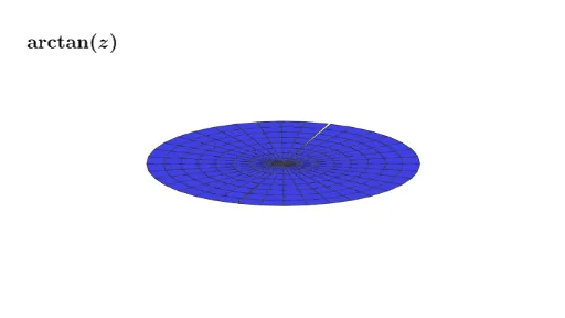
This GeoGebra example constructs a three-dimensional Riemann surface for the complex arctangent function arctan(z), visually demonstrating its multi-valued nature and branch structure. The core mathematical concepts include complex analysis, multi-valued functions, Riemann surfaces, branch points, and principal branches. The construction uses the Surface command along with buttons, sliders (t, a, b, c), and text objects to generate separate surfaces for the real part (Re) and imaginary part (Im), then layers multiple branches via objects like RSRe, RSIm, and their variants to create a spiral-like multi-sheet surface. This is ideal for university-level complex analysis courses, serving as a powerful teaching tool for instructors and a self-study aid for students to grasp how multi-valued functions are geometrically resolved into single-valued Riemann surfaces.
GeoGebra Commands & Parameters
Surface((u * cos(v)), (u * sin(v)), Re((u * cos(v)), (u * sin(v))), u, 0, 2, v, (-π), π - π / 200) → RSReSurface((u * cos(v)), (u * sin(v)), Re((u * cos(v)), (u * sin(v))), u, 0, 2, v, ((-π)) / 2, π / 2 - π / 300) → RSRe1Surface((u * cos(v)), (u * sin(v)), Re((u * cos(v)), (u * sin(v))), u, 0, 2, v, π / 2 + π / 300, (3 * π / 2) - π / 300) → RSRe2Surface((u * cos(v)), (u * sin(v)), (0 * (1 - t / 2)) + (Im((u * cos(v)), (u * sin(v))) * t / 2), u, 0, 2, v, (-π), π - π / 300) → RSImSurface((u * cos(v)), (u * sin(v)), (0 * (1 - t)) + (Re((u * cos(v)), (u * sin(v))) * If[0 ≤ t ≤ 1, t, 1]) + (0 * (2 - t)) + ((π * (0 - 2)) * (1 - t)), u, 0, 2, v, ((-π)) / 2, π / 2 - π / 300) → B0Surface((u * cos(v)), (u * sin(v)), (0 * (1 - t)) + (Re((u * cos(v)), (u * sin(v))) * If[0 ≤ t ≤ 1, t, 1]) + (0 * (2 - t)) + ((π * (1 - 2)) * (1 - t)), u, 0, 2, v, ((-π)) / 2, π / 2 - π / 300) → B1Surface((u * cos(v)), (u * sin(v)), (0 * (1 - t)) + (Re((u * cos(v)), (u * sin(v))) * If[0 ≤ t ≤ 1, t, 1]) + (0 * (2 - t)) + (0 * (1 - t)), u, 0, 2, v, ((-π)) / 2, π / 2 - π / 300) → B2Surface((u * cos(v)), (u * sin(v)), (0 * (1 - t)) + (Re((u * cos(v)), (u * sin(v))) * If[0 ≤ t ≤ 1, t, 1]) + (0 * (2 - t)) + ((π * (3 - 2)) * (1 - t)), u, 0, 2, v, ((-π)) / 2, π / 2 - π / 300) → B3Surface((u * cos(v)), (u * sin(v)), (0 * (1 - t)) + (Re((u * cos(v)), (u * sin(v))) * If[0 ≤ t ≤ 1, t, 1]) + (0 * (2 - t)) + ((π * (4 - 2)) * (1 - t)), u, 0, 2, v, ((-π)) / 2, π / 2 - π / 300) → B4Surface((u * cos(v)), (u * sin(v)), (0 * (1 - t)) + (Re((u * cos(v)), (u * sin(v))) * If[0 ≤ t ≤ 1, t, 1]) + (0 * (2 - t)) + ((π * (0 - 2)) * (1 - t)), u, 0, 2, v, π / 2 + π / 300, (3 * π / 2) - π / 300) → C0Surface((u * cos(v)), (u * sin(v)), (0 * (1 - t)) + (Re((u * cos(v)), (u * sin(v))) * If[0 ≤ t ≤ 1, t, 1]) + (0 * (2 - t)) + ((π * (1 - 2)) * (1 - t)), u, 0, 2, v, π / 2 + π / 300, (3 * π / 2) - π / 300) → C1Surface((u * cos(v)), (u * sin(v)), (0 * (1 - t)) + (Re((u * cos(v)), (u * sin(v))) * If[0 ≤ t ≤ 1, t, 1]) + (0 * (2 - t)) + (0 * (1 - t)), u, 0, 2, v, π / 2 + π / 300, (3 * π / 2) - π / 300) → C2Surface((u * cos(v)), (u * sin(v)), (0 * (1 - t)) + (Re((u * cos(v)), (u * sin(v))) * If[0 ≤ t ≤ 1, t, 1]) + (0 * (2 - t)) + ((π * (3 - 2)) * (1 - t)), u, 0, 2, v, π / 2 + π / 300, (3 * π / 2) - π / 300) → C3Surface((u * cos(v)), (u * sin(v)), (0 * (1 - t)) + (Re((u * cos(v)), (u * sin(v))) * If[0 ≤ t ≤ 1, t, 1]) + (0 * (2 - t)) + ((π * (4 - 2)) * (1 - t)), u, 0, 2, v, π / 2 + π / 300, (3 * π / 2) - π / 300) → C4
AI Drawing Prompt Reference
Create a 3D Riemann surface visualizing the multi-valued complex arctangent function. Use polar coordinates with radial distance from 0 to 2 and full angular coverage. The surface consists of multiple spiral-like sheets, each representing a branch. Construct separate surfaces for the real and imaginary parts: the real part is continuous and smooth, while the imaginary part uses a parameter t to transition from zero to its value, creating layered structures. Within angular intervals, add integer multiples of π as vertical offsets to generate parallel branches, forming a stepped or spiral tower. The overall shape resembles a rotating staircase, illustrating how a multi-valued function unfolds into single-valued sheets.
The prompt above was compiled from the original drawing commands and is for reference only.