
Rhombus Zolkowski
Loading the math board and drawing, please wait…
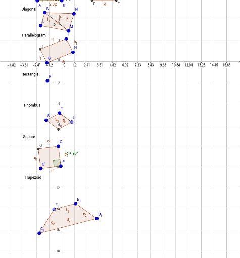
This example demonstrates the construction of the Rhombus Zolkowski. Key mathematical concepts include the properties of a rhombus, angles, and trigonometry. Using GeoGebra commands such as Polygon, Angle, Rotate, etc., the dynamic transformation and properties of the rhombus are showcased. Suitable for middle school and above students to learn about geometric transformations and properties of rhombuses.
GeoGebra Commands & Parameters
Polygon(A, B, C) → poly1, c, a, bAngle(C, B, A) → αAngle(A, C, B) → βAngle(B, A, C) → γLine(A, B) → fLine(C, f) → gPoint(g) → DLine(D, a) → hLine(D, b) → iIntersect(i, f) → EIntersect(h, f) → FPolygon(D, E, F) → poly2, f_1, d, eLine(G, H) → jLine(I, j) → kLine(H, I) → lLine(G, l) → mIntersect(m, k) → JPolygon(I, J, G, H) → poly3, i_1, j_1, g_1, h_1Polygon(L, K, N, M) → poly4, l_1, k_1, n, m_1Segment(K, M) → pLine(O, P) → qRotate(O, 90°, P) → O'Angle(O, P, O') → δLine(O', q) → rLine(P, O') → sLine(O, s) → tIntersect(t, r) → QPolygon(P, O, Q, O') → poly5, p_1, o, q_1, o'Line(C_1, D_1) → e_1Line(E_1, e_1) → f_2Point(f_2) → F_1Line(C_1, F_1) → g_2Line(D_1, E_1) → h_2Polygon(D_1, C_1, F_1, E_1) → poly8, d_2, c_2, f_3, e_2Line(G_1, H_1) → i_2Line(G_1, I_1) → j_2OrthogonalLine(H_1, j_2) → k_2Line(I_1, i_2) → l_2Line(H_1, I_1) → m_2Line(G_1, m_2) → n_2Intersect(n_2, l_2) → J_1Intersect(k_2, l_2) → K_1Segment(L_1, M_1) → p_2Line(M_1, N_1) → q_2Line(L_1, N_1) → r_2OrthogonalLine(M_1, r_2) → g_3Line(N_1, p_2) → h_3Line(L_1, q_2) → i_3Intersect(g_3, i_3) → P_1Intersect(g_3, h_3) → O_1Intersect(i_3, g_3) → Q_1Polygon(M_1, O_1, N_1) → poly6, n_3, m_3, o_1Line(S, T) → n_1Point(Circle[T, Distance[S, T]]) → USegment(T, U) → r_1Line(U, n_1) → s_1Line(S, r_1) → t_1Intersect(t_1, s_1) → VPolygon(S, T, U, V) → poly9, s_2, t_2, u, v