
Relativistic vs Galilean Velocity Addition
Loading the math board and drawing, please wait…
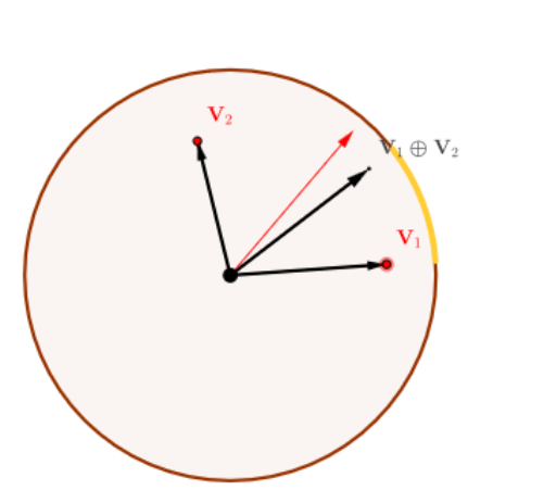
This example illustrates the difference between relativistic and Galilean velocity addition. Key mathematical concepts include vector addition. Using GeoGebra commands such as Circle, Segment, Vector, etc., the geometric meaning of different velocity additions is demonstrated. Suitable for high school physics and mathematics courses.
GeoGebra Commands & Parameters
Circle(A, 3) → cSegment(A, B) → fVector(A, B) → uSegment(A, C) → gVector(A, C) → vOrthogonalLine(A, u, xOyPlane) → hOrthogonalLine(B, u, xOyPlane) → iIntersect(h, c, 1) → DIntersect(i, c, 2) → ELine(D, E) → jIntersect(h, c, 2) → FIntersect(i, c, 1) → GLine(F, G) → kIntersect(j, k) → HOrthogonalLine(A, v, xOyPlane) → lOrthogonalLine(C, v, xOyPlane) → mIntersect(m, c, 1) → IIntersect(l, c, 2) → JLine(I, J) → nIntersect(m, c, 2) → KIntersect(l, c, 1) → LLine(K, L) → pIntersect(n, g) → MLine(B, A) → qLine(C, A) → rCircle(A, M, xOyPlane) → dIntersect(r, d, 2) → NIntersect(c, q, 2) → OIntersect(c, q, 1) → PCircle(O, M, P) → eIntersect(r, d, 1) → WLine(W, H) → sIntersect(s, c, 2) → QIntersect(s, c, 1) → RCircle(Q, A, R) → tIntersect(e, t, 2) → SLine(A, S) → aOrthogonalLine(A, a, xOyPlane) → bIntersect(b, c, 1) → TLine(T, S) → f_1Intersect(f_1, c, 1) → ULine(U, b) → g_1Intersect(a, g_1) → VVector(A, V) → wLine(P, M) → h_1Line(B, h_1) → i_1Intersect(r, i_1) → ZLine(O, Z) → j_1Intersect(j_1, c, 1) → A_1CircleArc(A, P, A_1, xOyPlane) → c_1Line(C, u) → k_1Line(B, v) → l_1Intersect(k_1, l_1) → B_1Line(A, B_1) → m_1Vector(A, B_1) → u_1