
Rate of Change of Linear Function Exercise
Loading the math board and drawing, please wait…
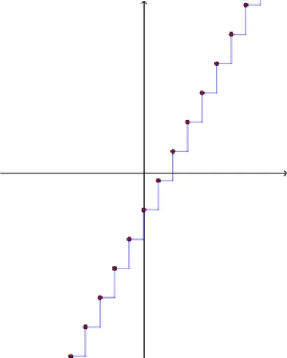
This example demonstrates the calculation and visualization of the rate of change (slope) of a linear function; involves core math concepts: linear functions, slope, coordinate geometry; constructed using GeoGebra commands/objects like Random, Line, Textfield, Polygon, LaTeX, Sequence, TableText; suitable for high school mathematics teaching to understand the relationship between function graphs and slopes.
GeoGebra Commands & Parameters
Random(-10, 10) → n_1Line(B, A) → aTextfield(deltay) → InputBox2Random(-5, 5) → mRandom(-10, 10) → nTextfield(b) → InputBox3Textfield(g) → InputBox1Polygon(C, D, E, F) → poly1, c_1, d, e, f_1LaTeX(deltax_1, true, true) → text10LaTeX(intersecty, true, true) → text11LaTeX(deltay_1, true, true) → text12Sequence(((deltax * i), intersecty + (deltay_1 * i)), i, -20, 20) → list1Sequence(Segment[A + ((deltax * (i + 1)), (deltay_1 * i)), A + ((deltax * (i + 1)), (deltay_1 * (i + 1)))], i, -20, 20) → risesSequence(Segment[A + ((deltax * i), (deltay_1 * i)), A + ((deltax * (i + 1)), (deltay_1 * i))], i, -20, 20) → runsTextfield(i) → InputBox4LaTeX(deltax, true, true) → text6Random(-3, 3) → jTableText({{p, k, k_1}, {A2, B2, C2}, {A3, B3, C3}, {A4, B4, C4}, {A5, B5, C5}, {A6, B6, C6}, {A7, B7, C7}, {A8, B8, C8}}, "|_lll") → text2