Quadratic Roots and y-Intercepts

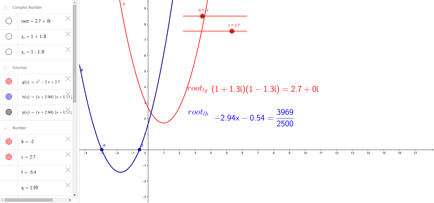
This GeoGebra example visualizes the relationship between the roots of a quadratic function and its y-intercept, demonstrating how the graph interacts with the x-axis and y-axis as coefficients change. Core mathematical concepts include quadratic function properties, discriminant analysis, the nature of real and complex roots, and the geometric interpretation of complex solutions. Construction employs GeoGebra commands such as Point, Root, Expand, ComplexRoot, and FractionText, with dynamic coefficients b and c displayed via input sliders. Root values are shown as exact text or fractions, and complex roots are represented geometrically on the complex plane. The example is suitable for high school algebra and pre-calculus courses, helping students connect algebraic solutions with graphical behavior and understand the transition from real to complex roots.