
Probability of Existence of a Rectangle
Loading the math board and drawing, please wait…
In collections
Pi Approximations
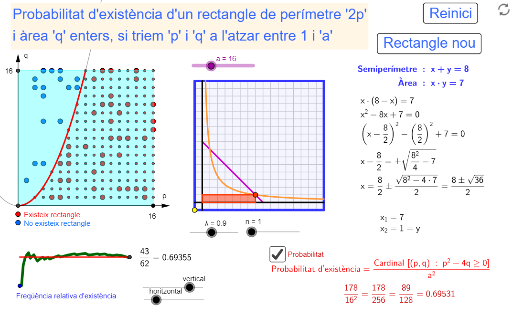
This example demonstrates the probability of the existence of a rectangle given a perimeter of 2p and an area of q as integers. Key mathematical concepts include probability and geometry. Using GeoGebra commands such as Vector, Intersect, and Polygon, the conditions for the existence of a rectangle are constructed. Suitable for middle school and above students learning geometric probability.
GeoGebra Commands & Parameters
Vector(((-λ), (-λ)), J) → uIntersect(f, xAxis, 1) → APolygon(A, B, 4) → Polígon1, a_1, b, c, d, C, DIntersect(f, c, 1) → ESequence(Sequence[(p, k), k, 1, p^(2) / 4 - 1 / 8 + (-1)^(p) / 8], p, 1, t) → llista1Sequence(Sequence[(k, h), h, 1, a], k, floor(t) + 1, a) → llista2GCD(S1, a^(2)) → jTranslate(Polygon[((-λ), (-λ)), (((n * a) * λ), (-λ)), 4], u) → Polígon2Translate(fs, u) → tfsTranslate(Segment[(0, (-λ)), (0, ((n * a) * λ))], u) → e2Translate(fp, u) → tfpTranslate(((λ * (p + (p^(2) - (4 * q))^(0.5)) / 2), (λ * (p - (p^(2) - (4 * q))^(0.5)) / 2)), u) → FTranslate(Segment[((-λ), 0), (((n * a) * λ), 0)], u) → e1OrthogonalLine(F, e1) → hOrthogonalLine(F, e2) → iIntersect(h, e1) → GIntersect(i, e2) → HIntersect(e1, e2) → IPolygon(H, F, G, I) → Polígon3, h_1, f_1, g_1, i_1Sequence(Translate[Segment[((k * λ), (-λ)), ((k * λ), ((n * a) * λ))], u], k, 1, (n * a)) → se2Sequence(Translate[Segment[((-λ), (k * λ)), (((n * a) * λ), (k * λ))], u], k, 1, (n * a)) → se1RemoveUndefined(LC) → LC2Length(LC) → tirLength(LC2) → tircPolyLine(K + Append[(0, 0), Sequence[(HF * Element[LR, j]), j, 1, Length[LR]]]) → LR2Vector(A, B + (2, 0)) → vVector(A, D + (0, 2)) → wCentroid(Polígon2) → CPRemoveUndefined(LI) → LI2Segment(K + (0, (h1 * S1 / a^(2))), K + ((h2 * (Length[LR] - 1)), (h1 * S1 / a^(2)))) → lPointList(LC2) → LC3
AI Drawing Prompt Reference
This is a geometric figure about the probability of a rectangle's existence. The figure includes a rectangle and a square, showing their side lengths and area relationships to illustrate probability calculations. The construction order starts with the rectangle, then adds the square, and finally uses intersections and transformations to show their relationships. The elements include the rectangle, square, intersection points, and related line segments, presenting a clear representation of geometric probability.
The prompt above was compiled from the original drawing commands and is for reference only.