
Position, Velocity, and Acceleration vs. Time Graphs
Loading the math board and drawing, please wait…
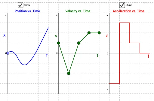
This example demonstrates how changes in a velocity-time graph affect the corresponding position-time and acceleration-time graphs. It covers basic calculus concepts such as derivatives and integrals. GeoGebra commands used include slider animation, locus, and function graphing. Suitable for high school and above students.
GeoGebra Commands & Parameters
Segment(A, B) → a_3Point(a_3) → RSegment((5, -4), (5, 4)) → m1Point(m1) → ESegment((6, -4), (6, 4)) → m2Point(m2) → FSegment(E, F) → aSegment((9, -4), (9, 4)) → m5Segment((8, -4), (8, 4)) → m4Segment((7, -4), (7, 4)) → m3Midpoint(a_3) → DSegment(D, C) → bSegment(A_1, B_1) → a_1Midpoint(a_1) → D_1Segment(D_1, C_1) → b_1Segment(A_2, B_2) → a_2Midpoint(a_2) → D_2Segment(D_2, C_2) → b_2Point(m3) → GSegment(F, G) → cPoint(m4) → HSegment(G, H) → dPoint(m5) → ISegment(H, I) → eSegment(J, K) → fSegment(K, L) → gSegment(L, M) → hSegment(M, N) → iSegment(N, O) → jSegment(O, P) → kSegment(P, Q) → l
AI Drawing Prompt Reference
Draw a velocity-time graph where velocity is 0 at 5 seconds and 6 seconds, then draw position-time and acceleration-time graphs. The slope of the velocity graph corresponds to changes in the position graph, and the slope of the position graph corresponds to changes in the acceleration graph. Use slider animation to change the velocity graph and observe the changes in the position and acceleration graphs.
The prompt above was compiled from the original drawing commands and is for reference only.