Polynomials: Exploring the y-axis Intercept when x=0

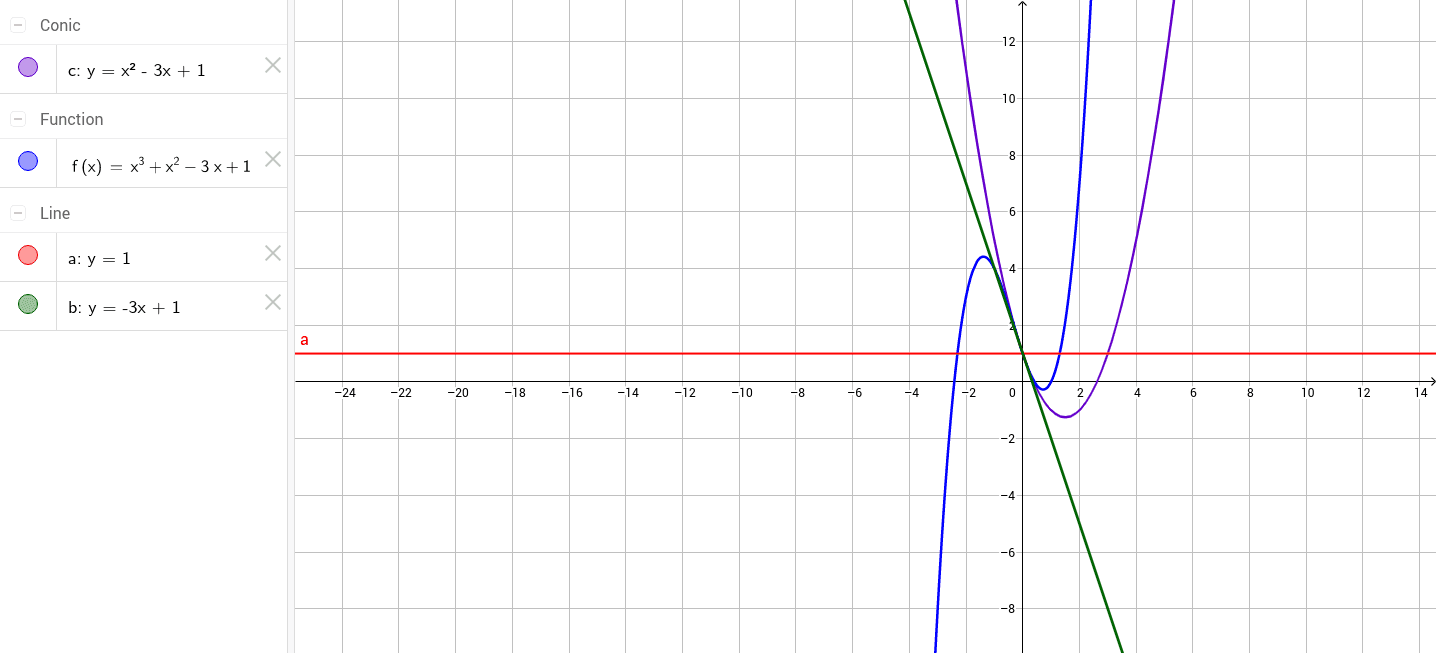
This GeoGebra example dynamically demonstrates the y-axis intercept of a polynomial function, i.e., the value of the function when x=0. The core mathematical concept is the intersection of a function graph with the coordinate axes, polynomial evaluation, and the geometric meaning of the intercept. The construction uses GeoGebra objects a, b, c, and f (likely parameters or function definitions) to define the polynomial f, allowing users to adjust parameters and observe how the intercept changes. Suitable for middle and high school students learning function graphs, coordinate geometry basics, or the connection between algebra and geometry. It is ideal for classroom demonstrations or self-guided exploration, helping learners understand the role of the constant term in the polynomial expression and its visual representation on the graph.