
Polynomial with Equidistant Roots
Loading the math board and drawing, please wait…
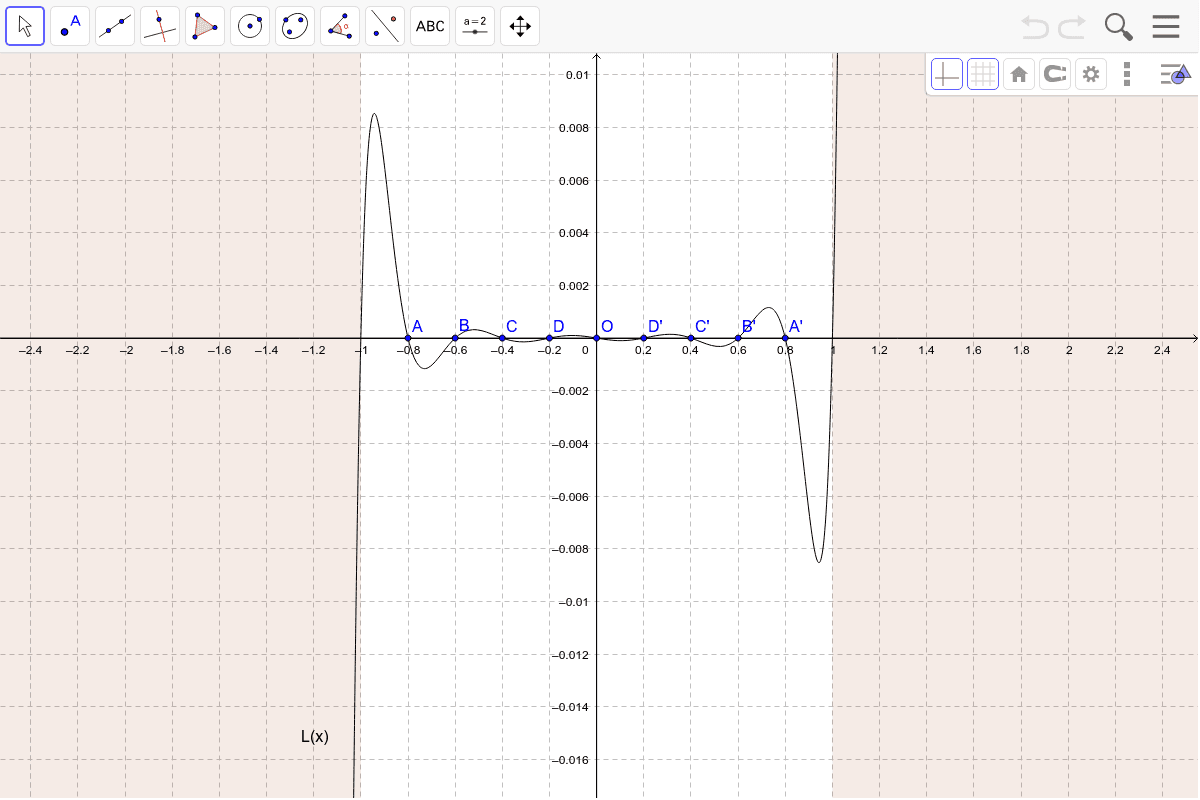
This example demonstrates the polynomial arising in the Lagrange interpolation error formula, where roots are default equidistant. Any shift reveals the error pattern. Core math concepts include polynomials, roots, interpolation error, and equidistant distribution. Constructed using GeoGebra commands like Point, Line, Polynomial, Polygon, Mirror, and objects such as i, K, E, d, f, g, a, B_1, etc. Suitable for high school and above, helping learners understand the relationship between interpolation error and root distribution dynamically.
GeoGebra Commands & Parameters
Point(xAxis) → KPoint(xAxis) → ELine(E, K) → dPolynomial((x + 1) * (x + 0.85) * (x + 0.6) * (x + 0.4) * (x + 0.2) * x * (x - 0.2) * (x - 0.4) * (x - 0.6) * (x - 0.85) * (x - 1)) → fPolynomial((x + 1) * (x + 0.8) * (x + 0.6) * (x + 0.4) * (x + 0.2) * x * (x - 0.2) * (x - 0.4) * (x - 0.6) * (x - 0.8) * (x - 1)) → gPolygon(B_1, C_1, E_1, F) → poly1, b, c, e, f_1Polygon(G, H, I, J) → poly2, g_1, h_1, i_1, jPoint(d) → BMirror(B, a) → B'Point(d) → CMirror(C, a) → C'Point(d) → DMirror(D, a) → D'Point(d) → AMirror(A, a) → A'Point(d) → OPolynomial((x + 1) * (x - x(A)) * (x - x(B)) * (x - x(C)) * (x - x(D)) * (x - x(O)) * (x - x(D')) * (x - x(C')) * (x - x(B')) * (x - x(A')) * (x - 1)) → h
AI Drawing Prompt Reference
Draw a polynomial function with equidistant roots and show its relationship with interpolation error. Start by plotting two points on the x-axis and connecting them to form a line. Based on this line, construct a polynomial with roots evenly distributed on the x-axis. Then create two polygons corresponding to the positive and negative roots of the polynomial. Next, reflect points across the line to obtain symmetric points. Finally, use these symmetric points and the original polynomial's roots to draw a new polynomial, illustrating the error pattern.
The prompt above was compiled from the original drawing commands and is for reference only.