
Polar Plotter
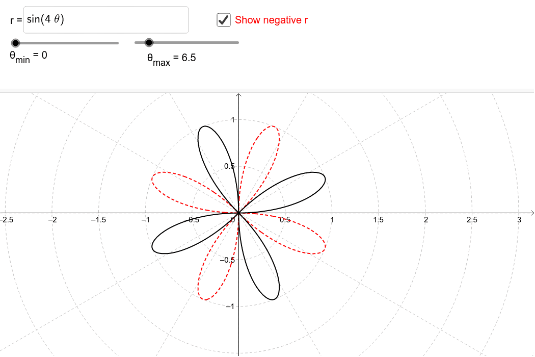
Loading the math board and drawing, please wait…
This example demonstrates how to plot polar equations using GeoGebra, showcasing the dynamic behavior of the graphs. Core math concepts include polar coordinate systems, function graphs, trigonometric functions, and parametric equations. Key GeoGebra commands and objects used are Textfield, Curve (polar), Cartesian, and r, f, g, h, inputBox1, θ_{max}, θ_{min}, b, a, c. Suitable for high school and above students to explore polar equations and their applications.
GeoGebra Commands & Parameters
Textfield(r) → inputBox1CurveCartesian((h(θ) * cos(θ)), (h(θ) * sin(θ)), θ, θ_{min}, θ_{max}) → bCurveCartesian((g(θ) * cos(θ)), (g(θ) * sin(θ)), θ, θ_{min}, θ_{max}) → a
AI Drawing Prompt Reference
Create a dynamic polar plot with an input box for entering a polar equation. Display two curves generated from different polar functions: one from function h and another from function g. Both curves are plotted by converting polar to Cartesian coordinates, with x-coordinate as the function value times cosine of the angle and y-coordinate as the function value times sine of the angle, over a range from minimum to maximum angle. The graph should illustrate the dynamic behavior of polar curves and highlight the relationship between trigonometric functions and parametric equations.
The prompt above was compiled from the original drawing commands and is for reference only.