
Plotting Integer Points in Linear Programming by STGSS-TSN
Loading the math board and drawing, please wait…
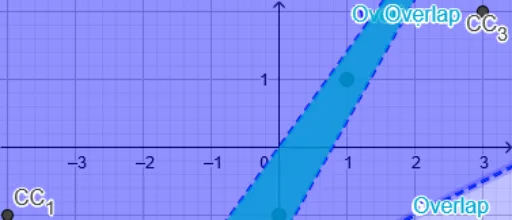
This example demonstrates how to plot all integer coordinate points within the feasible region of a linear programming problem, visually contrasting integer programming with continuous linear programming. Core mathematical concepts include linear programming, integer constraints, feasible regions, objective functions, and the discrete nature of integer points. Construction highlights: using GeoGebra commands such as Corner to obtain polygon vertices, Join to connect boundaries, and KeepIf to filter integer points satisfying constraints, with objects like b, C1-C4, CC1, CC3, a, c, IntegerPoints, Overlap, and Result. Suitable for high school or early college students learning linear programming and integer programming, helping them understand the existence of integer solutions and optimal solution locations.
GeoGebra Commands & Parameters
Corner(2) → C_{2}Corner(3) → C_{3}Corner(4) → C_{4}Corner(1) → C_{1}Join(Sequence[Sequence[(i, j), j, y(CC_{1}), y(CC_{3})], i, x(CC_{1}), x(CC_{3})]) → IntegerPointsKeepIf(IsInRegion[Q, Overlap], Q, IntegerPoints) → Result
AI Drawing Prompt Reference
Draw a feasible region as a polygon with a semi-transparent fill. Inside and on the boundary of this region, plot all integer-coordinate points (points with both x and y as integers) as solid dots, making them clearly visible against the continuous region. Outline the polygon boundary with thick lines. Highlight the subset of integer points that satisfy all constraints, distinguishing them from other integer points. The overall figure should illustrate the difference between integer and continuous linear programming, showing where integer optimal solutions may lie.
The prompt above was compiled from the original drawing commands and is for reference only.