
Photon Absorption/Ionization & Energy Level Diagrams
Loading the math board and drawing, please wait…
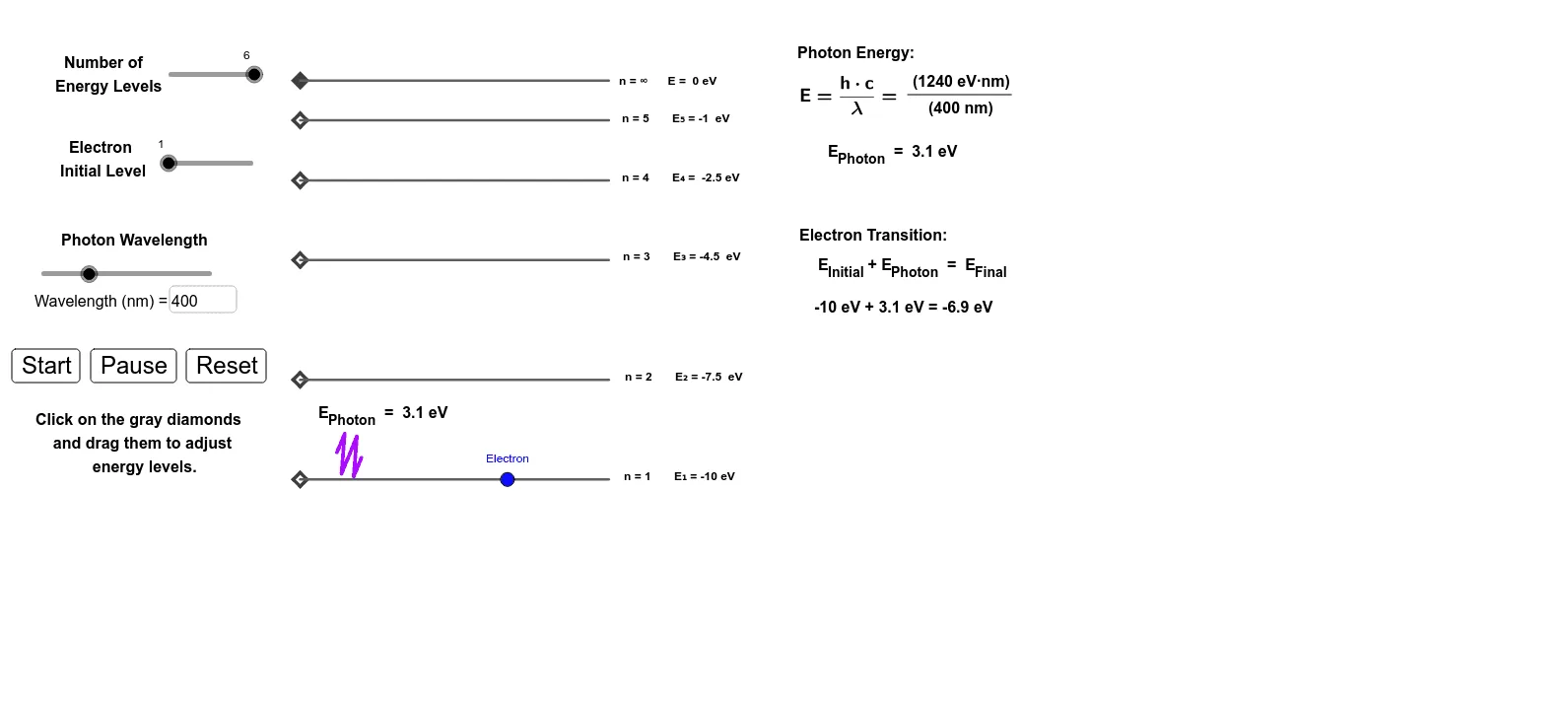
This GeoGebra example provides an interactive visualization of photon absorption, ionization, and atomic energy level transitions. It demonstrates how an electron jumps between discrete energy levels when the photon energy matches the energy difference, and how it escapes the atom when the photon energy exceeds the ionization threshold. The core mathematical concepts include energy conservation, discrete energy levels, the relation E=hν, and the use of geometric elements (lines, circles, polygons) to represent abstract physical quantities. The construction employs GeoGebra commands such as Line, Point, Circle, Segment, Polygon for building the energy axis and electron positions, If, Intersect, OrthogonalLine, Slope for conditional logic and geometric relations, sliders to control photon energy and time, and text fields to display numerical values. This resource is suitable for high school or introductory university physics courses covering atomic physics and quantum mechanics, as well as for interdisciplinary math-physics explorations.
GeoGebra Commands & Parameters
Line(R_2, M_2) → m_3Point(yAxis) → CPoint(yAxis) → BPoint(yAxis) → DPoint(yAxis) → EPoint(yAxis) → FIf(t < tcollide, 0, If[t > tcollide + ttransition, ttransition, t - tcollide]) → telectronIf(0 < leveli < 2, 1, 0) → testleveli1If(3 < leveli < 5, 1, 0) → testleveli4If(1 < leveli < 3, 1, 0) → testleveli2If(2 < leveli < 4, 1, 0) → testleveli3If(4 < leveli < 6, 1, 0) → testleveli5If(Energynew > (-r), 1, 0) → testAIf(abs(abs(Energynew) - abs(y(E))) < r, 1, 0) → testEIf(levelnumber > 5, 1, 0) → testlevel6If(abs(abs(Energynew) - abs(y(B))) < r, testlevel6, 0) → testBIf(levelnumber > 4, 1, 0) → testlevel5If(abs(abs(Energynew) - abs(y(C))) < r, testlevel5, 0) → testCIf(levelnumber > 3, 1, 0) → testlevel4If(abs(abs(Energynew) - abs(y(D))) < r, testlevel4, 0) → testDLine(P_2, m_3) → j_3Line(K_2, yAxis) → i_3Intersect(i_3, j_3) → T_2OrthogonalLine(M, m_3) → nIntersect(n, j_3) → PSlope(m_3) → slopephotonpathLine(A, xAxis) → fPoint(f) → KOrthogonalLine(K, f) → f_2Line(C, xAxis) → hIntersect(h, f_2) → O_1Segment(C, O_1) → i_2Segment(A, K) → g_2Line(F, xAxis) → kIntersect(k, f_2) → S_2Segment(F, S_2) → l_2Line(E, xAxis) → jIntersect(j, f_2) → Q_1Segment(E, Q_1) → k_2Line(D, xAxis) → iIntersect(i, f_2) → P_1Segment(D, P_1) → j_2Line(B, xAxis) → gIntersect(g, f_2) → N_1Segment(B, N_1) → h_2If(490 < w < 510, (-((w - 510) / 20)), If[380 < w < 491, 1, 0]) → BCoeffIf(440 < w < 490, (w - 440) / 50, If[580 < w < 645, (-((w - 645) / 65)), If[489 < w < 581, 1, 0]]) → GCoeffIf(380 < w < 440, (w - 440) / 60, If[510 < w < 580, (w - 510) / 70, If[579 < w < 780, 1, 0]]) → RCoeffLine(I_2, L_2) → p_3OrthogonalLine(J_2, m_3) → q_3OrthogonalLine(I_2, m_3) → r_3Circle(I_2, 1) → c_3Intersect(c_3, r_3) → N_2, O_2Intersect(q_3, j_3) → W_2Circle(W_2, 1) → d_3Intersect(d_3, q_3, 1) → Z_2Midpoint(Z_2, O_2) → A_3Midpoint(I_2, W_2) → B_3Midpoint(B_3, I_2) → C_3Midpoint(C_3, I_2) → D_3Midpoint(O_2, A_3) → E_3Midpoint(E_3, A_3) → F_3Midpoint(B_3, W_2) → G_3Midpoint(I_2, O_2) → I_3Midpoint(B_3, G_3) → J_3Midpoint(A_3, Z_2) → K_3Midpoint(K_3, Z_2) → L_3Midpoint(Z_2, W_2) → M_3PolyLine(I_3, D_3, F_3, J_3, L_3, M_3) → s_3If(t > tcollide, 1, 0) → testcollideIf(tcollide + ttransition < t, 1, 0) → testtimeionizeTextfield(w) → InputBox1If(abs(Energyphoton) > abs(electroni), (-electroni), Energyphoton) → transitionarrowVector(G, H) → uSegment(I, J) → lCircle(P, 1) → dCircle(L, 1) → cOrthogonalLine(L, m_3) → mIntersect(c, m, 1) → NIntersect(d, n, 1) → OMidpoint(L, P) → QMidpoint(N, O) → RMidpoint(L, N) → SMidpoint(P, O) → TMidpoint(L, Q) → UMidpoint(L, U) → VMidpoint(N, R) → WMidpoint(W, R) → ZMidpoint(Q, P) → A_1Midpoint(Q, A_1) → B_1Midpoint(R, O) → C_1Midpoint(C_1, O) → D_1PolyLine(S, V, Z, B_1, D_1, T) → pPolygon(E_1, F_1, G_1, H_1) → poly1, e_1, f_1, g_1, h_1