
Photon Absorption/Ionization & Energy Level Diagrams by Barb Newitt (2)
Loading the math board and drawing, please wait…
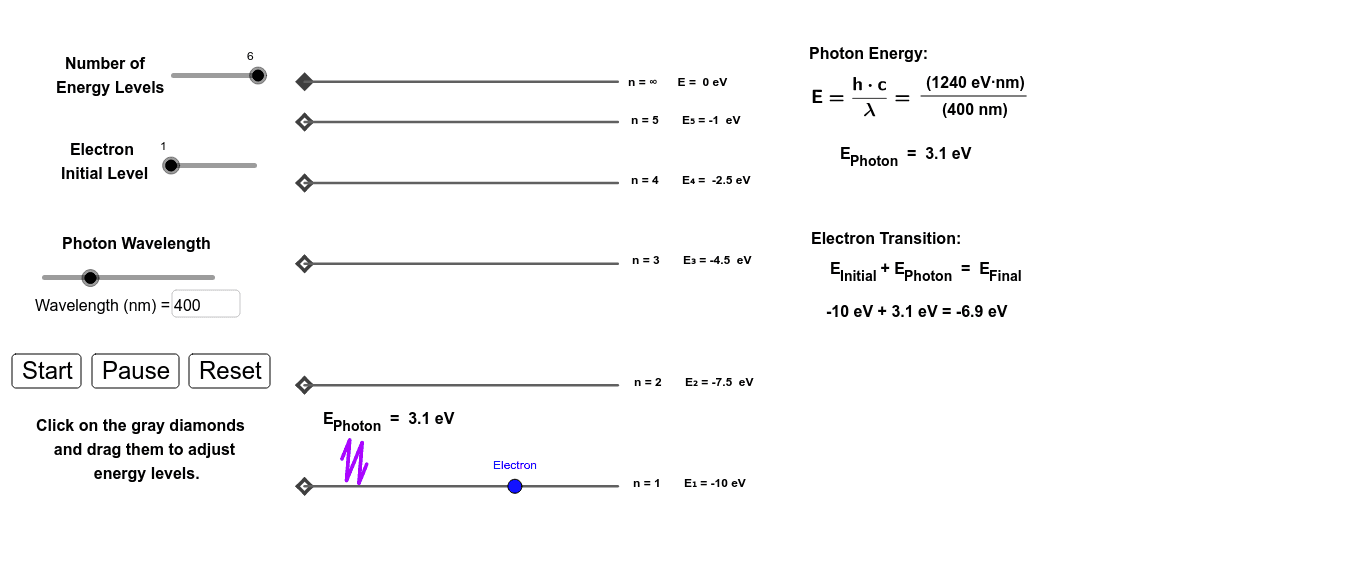
This example demonstrates the dynamic visualization of photon absorption, ionization, and atomic energy level transitions. It involves core mathematical concepts such as coordinate systems, geometric constructions, inequality representation, and vector operations. GeoGebra commands and objects like Line, Point, If, Intersect, OrthogonalLine, Slope, Segment, Circle, Midpoint, PolyLine, Textfield, Vector, Polygon are utilized in its construction. Suitable for high school physics and university-level introductory physics education, helping visualize atomic energy levels and quantum transitions.
GeoGebra Commands & Parameters
Line(R_2, M_2) → m_3Point(yAxis) → CPoint(yAxis) → BPoint(yAxis) → DPoint(yAxis) → EPoint(yAxis) → FIf(t < tcollide, 0, If[t > tcollide + ttransition, ttransition, t - tcollide]) → telectronIf(0 < leveli < 2, 1, 0) → testleveli1If(3 < leveli < 5, 1, 0) → testleveli4If(1 < leveli < 3, 1, 0) → testleveli2If(2 < leveli < 4, 1, 0) → testleveli3If(4 < leveli < 6, 1, 0) → testleveli5If(Energynew > (-r), 1, 0) → testAIf(abs(abs(Energynew) - abs(y(E))) < r, 1, 0) → testEIf(levelnumber > 5, 1, 0) → testlevel6If(abs(abs(Energynew) - abs(y(B))) < r, testlevel6, 0) → testBIf(levelnumber > 4, 1, 0) → testlevel5If(abs(abs(Energynew) - abs(y(C))) < r, testlevel5, 0) → testCIf(levelnumber > 3, 1, 0) → testlevel4If(abs(abs(Energynew) - abs(y(D))) < r, testlevel4, 0) → testDLine(P_2, m_3) → j_3Line(K_2, yAxis) → i_3Intersect(i_3, j_3) → T_2OrthogonalLine(M, m_3) → nIntersect(n, j_3) → PSlope(m_3) → slopephotonpathLine(A, xAxis) → fPoint(f) → KOrthogonalLine(K, f) → f_2Line(C, xAxis) → hIntersect(h, f_2) → O_1Segment(C, O_1) → i_2Segment(A, K) → g_2Line(F, xAxis) → kIntersect(k, f_2) → S_2Segment(F, S_2) → l_2Line(E, xAxis) → jIntersect(j, f_2) → Q_1Segment(E, Q_1) → k_2Line(D, xAxis) → iIntersect(i, f_2) → P_1Segment(D, P_1) → j_2Line(B, xAxis) → gIntersect(g, f_2) → N_1Segment(B, N_1) → h_2If(490 < w < 510, (-((w - 510) / 20)), If[380 < w < 491, 1, 0]) → BCoeffIf(440 < w < 490, (w - 440) / 50, If[580 < w < 645, (-((w - 645) / 65)), If[489 < w < 581, 1, 0]]) → GCoeffIf(380 < w < 440, (w - 440) / 60, If[510 < w < 580, (w - 510) / 70, If[579 < w < 780, 1, 0]]) → RCoeffLine(I_2, L_2) → p_3OrthogonalLine(J_2, m_3) → q_3OrthogonalLine(I_2, m_3) → r_3Circle(I_2, 1) → c_3Intersect(c_3, r_3) → N_2, O_2Intersect(q_3, j_3) → W_2Circle(W_2, 1) → d_3Intersect(d_3, q_3, 1) → Z_2Midpoint(Z_2, O_2) → A_3Midpoint(I_2, W_2) → B_3Midpoint(B_3, I_2) → C_3Midpoint(C_3, I_2) → D_3Midpoint(O_2, A_3) → E_3Midpoint(E_3, A_3) → F_3Midpoint(B_3, W_2) → G_3Midpoint(I_2, O_2) → I_3Midpoint(B_3, G_3) → J_3Midpoint(A_3, Z_2) → K_3Midpoint(K_3, Z_2) → L_3Midpoint(Z_2, W_2) → M_3PolyLine(I_3, D_3, F_3, J_3, L_3, M_3) → s_3If(t > tcollide, 1, 0) → testcollideIf(tcollide + ttransition < t, 1, 0) → testtimeionizeTextfield(w) → InputBox1If(abs(Energyphoton) > abs(electroni), (-electroni), Energyphoton) → transitionarrowVector(G, H) → uSegment(I, J) → lCircle(P, 1) → dCircle(L, 1) → cOrthogonalLine(L, m_3) → mIntersect(c, m, 1) → NIntersect(d, n, 1) → OMidpoint(L, P) → QMidpoint(N, O) → RMidpoint(L, N) → SMidpoint(P, O) → TMidpoint(L, Q) → UMidpoint(L, U) → VMidpoint(N, R) → WMidpoint(W, R) → ZMidpoint(Q, P) → A_1Midpoint(Q, A_1) → B_1Midpoint(R, O) → C_1Midpoint(C_1, O) → D_1PolyLine(S, V, Z, B_1, D_1, T) → pPolygon(E_1, F_1, G_1, H_1) → poly1, e_1, f_1, g_1, h_1
AI Drawing Prompt Reference
Draw a diagram showing atomic energy level transitions. Include circles representing different energy levels, connected by line segments. Add arrows indicating photon absorption and ionization processes, and horizontal lines representing energy thresholds. The diagram should clearly show the relationships between energy levels to help understand quantum energy conversion concepts.
The prompt above was compiled from the original drawing commands and is for reference only.