
Phantom Graph of x(x-3)^2
Loading the math board and drawing, please wait…
In collections
Phantom Graphs
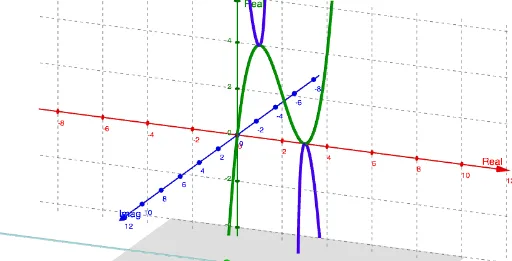
This example demonstrates the phantom graph of the function x(x-3)^2. The core mathematical concepts involved include the complex roots of quadratic equations. Using GeoGebra commands such as ComplexRoot and CurveCartesian, the phantom graph can be constructed. Suitable for high school mathematics education, particularly in coordinate geometry and complex numbers.
GeoGebra Commands & Parameters
ComplexRoot(f(x) - c) → z_1, z_2, z_3CurveCartesian(t, (-8 * t^(3)) + (48 * t^(2)) - (90 * t) + 54, sqrt((3 * t^(2)) - (12 * t) + 9), t, 3, 25) → eCurveCartesian(t, (-8 * t^(3)) + (48 * t^(2)) - (90 * t) + 54, (-sqrt((3 * t^(2)) - (12 * t) + 9)), t, 3, 25) → jCurveCartesian(t, (-8 * t^(3)) + (48 * t^(2)) - (90 * t) + 54, (-sqrt((3 * t^(2)) - (12 * t) + 9)), t, -25, 1) → dCurveCartesian(t, (-8 * t^(3)) + (48 * t^(2)) - (90 * t) + 54, sqrt((3 * t^(2)) - (12 * t) + 9), t, -25, 1) → b
AI Drawing Prompt Reference
Draw the phantom graph of the function x(x-3)^2. Start with the real cubic curve, then add two symmetric branches above and below it, derived from the complex roots. These branches extend from the real curve, forming a ghost-like shape. Use a parameter t to define four parametric curves with the same x-coordinate but y-coordinates as positive and negative square roots, covering t from -25 to 25 in two segments each. The result shows the main curve with symmetric extensions illustrating the complex roots.
The prompt above was compiled from the original drawing commands and is for reference only.