
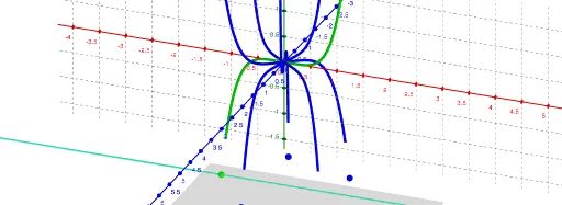
Phantom Graph for f(x)=x^5
Loading the math board and drawing, please wait…
In collections
Phantom Graphs
This example demonstrates the phantom graph of the function f(x)=x^5. It involves the concept of complex numbers, and uses GeoGebra commands such as ComplexRoot, Plane, Ray, Circle, and CurveCartesian to visually understand the relationship between complex roots and the function graph. Suitable for high school mathematics education, particularly in coordinate geometry and complex numbers.
GeoGebra Commands & Parameters
ComplexRoot(f(x) - c) → z_1, z_2, z_3, z_4, z_5Plane((0, c, 9), (1, c, 0), (0, c, 1)) → hRay((0, 0), (1; (2 * π / 5))) → iRay((0, 0), (1; (4 * π / 5))) → jRay((0, 0), (1; (6 * π / 5))) → kRay((0, 0), (1; (8 * π / 5))) → lRay((0, 0), (1; π / 5)) → mRay((0, 0), (1; (3 * π / 5))) → nRay((0, 0), (1; (7 * π / 5))) → pRay((0, 0), (1; (9 * π / 5))) → qCircle((0, 0), z_1) → rCurveCartesian((c^(1 / 5) * (-1 + sqrt(5)) / 4), c, (c^(1 / 5) * sqrt((5 + sqrt(5)) / 8)), c, -25, 25) → oaCurveCartesian((c^(1 / 5) * (-1 - sqrt(5)) / 4), c, (c^(1 / 5) * sqrt((5 - sqrt(5)) / 8)), c, -25, 25) → oeCurveCartesian((c^(1 / 5) * (-1 + sqrt(5)) / 4), c, ((-c^(1 / 5)) * sqrt((5 + sqrt(5)) / 8)), c, -25, 25) → obCurveCartesian(t, (t^(5) * (176 + (80 * sqrt(5)))), (t * sqrt(5 + (2 * sqrt(5)))), t, -25, 25) → aCurveCartesian(t, (t^(5) * (176 + (80 * sqrt(5)))), ((-t) * sqrt(5 + (2 * sqrt(5)))), t, -25, 25) → bCurveCartesian(t, (t^(5) * (176 - (80 * sqrt(5)))), (t * sqrt(5 - (2 * sqrt(5)))), t, -25, 25) → dCurveCartesian(t, (t^(5) * (176 - (80 * sqrt(5)))), ((-t) * sqrt(5 - (2 * sqrt(5)))), t, -25, 25) → e
AI Drawing Prompt Reference
Draw the phantom graph of the function f(x)=x^5. First, find the five complex roots of the function. Then, draw five circles centered at the origin with these roots as radii. Next, draw eight rays starting from the origin with angles π/5, 2π/5, 3π/5, 4π/5, 6π/5, 7π/5, 8π/5, and 9π/5. Finally, use the CurveCartesian command to draw four curves representing the real and imaginary parts of the function.
The prompt above was compiled from the original drawing commands and is for reference only.