Perimeter Testing 1: Parallelogram Perimeter and Random Experiments

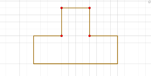
①This GeoGebra example dynamically demonstrates perimeter measurement of a parallelogram combined with random experiments, visually showing how perimeter relates to side lengths and diagonals. ②Core mathematical concepts include properties of parallelograms, perimeter calculation, random experiments (possibly Monte Carlo methods), and indefinite integrals as a background notion. ③Construction highlights: using Point, Segment, and Line commands to create points (A, B, C, D, etc.) and segments (f, g, h, etc.), constructing a parallelogram via parallel lines, and incorporating random points for perimeter testing. ④Suitable for middle school geometry to explore perimeter variations, or for introductory probability experiments, and as a dynamic geometry demonstration for beginners.