
Percentage Change Demonstration by Anthony OR 柯志明
Loading the math board and drawing, please wait…
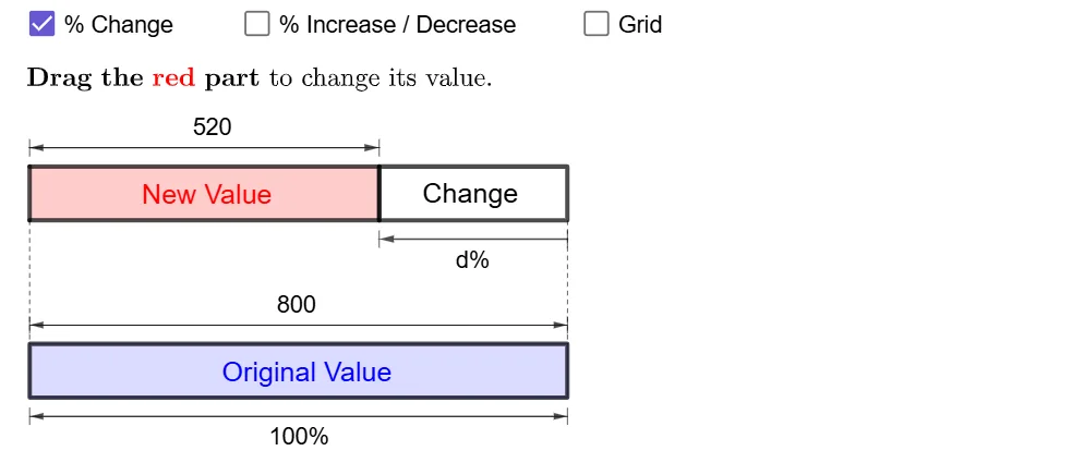
This example demonstrates how to construct dynamic geometric visualizations of percentage change using GeoGebra. It involves core math concepts like percentage calculations, algebraic operations, and geometric transformations. Key GeoGebra commands used include If, Point, Polygon, Sequence, Textfield, Segment, and Vector. Suitable for high school mathematics education to understand the application of percentage change in geometry and algebra.
GeoGebra Commands & Parameters
If(a, "d", ((If[p ∧ x(P) < 10, "−", If[p ∧ x(P) > 10, "+"]] * abs(d)) * "")) → dtextIf(c', "n", (n * "")) → ntextPoint(yAxis) → APoint(yAxis) → BIf(x(P) ≤ 10, A + (10, 0), B + (10, 0)) → A0If(x(P) ≤ 10, P, (x(P), y(B))) → P0Polygon(P, Q, (0, y(Q)), (0, y(P))) → q1, p_1, q_1, g, hPolygon({P0, A0, A0 + (0, 1), P0 + (0, 1)}) → q2Polygon({B, B + (10, 0), B + (10, 1), B + (0, 1)}) → q3Polygon({B, B + (10, 0), B + (10, 1), B + (0, 1)}) → q4Sequence(Segment[B + (i, 0), B + (i, 1)], i, 1, 9, 1) → l1Sequence(Sequence[Segment[B + (j + i, 0), B + (j + i, 1)], j, 0, 9, 1], i, 0.1, 0.9, 0.1) → l2Sequence(Segment[A + (i, 0), A + (i, 1)], i, 1, 9, 1) → l3Sequence(Sequence[Segment[A + (j + i, 0), A + (j + i, 1)], j, 0, 9, 1], i, 0.1, 0.9, 0.1) → l4Textfield(n) → InputBox1Textfield(m) → InputBox2If(b, "m", (m * "")) → mtextSegment(If[b_1 ≟ 0, A, A0] + (0, 1.2), If[b_1 ≟ 0, A, A0] + (0, 1.5)) → iSegment(If[b_1 ≟ 0, P, P0] + (0, 1.2), If[b_1 ≟ 0, P, P0] + (0, 1.5)) → jVector(Midpoint[i], Midpoint[j]) → uVector(Midpoint[j], Midpoint[i]) → vSegment(A0 - (0, 0.2), A0 - (0, 0.5)) → kSegment(P0 - (0, 0.2), P0 - (0, 0.5)) → lVector(Midpoint[k], Midpoint[l]) → wVector(Midpoint[l], Midpoint[k]) → eSegment(B + (0, 1.2), B + (0, 1.5)) → fSegment(B + (10, 1.2), B + (10, 1.5)) → rVector(Midpoint[f], Midpoint[r]) → sVector(Midpoint[r], Midpoint[f]) → tSegment(B - (0, 0.2), B - (0, 0.5)) → f_1Segment(B + (10, -0.2), B + (10, -0.5)) → g_1Vector(Midpoint[f_1], Midpoint[g_1]) → u_1Vector(Midpoint[g_1], Midpoint[f_1]) → v_1If(a, "d", If[b, If[b_1 ≟ 0, "m", "c"], "n"]) → text12Sequence(Segment[A + (10 + i, 0), A + (10 + i, 1)], i, 0.1, x(P) - 10, 0.1) → l6Sequence(Segment[A + (10 + i, 0), A + (10 + i, 1)], i, 0, floor(x(P) - 10)) → l5Sequence(Segment[A0 + (i, 0), A0 + (i, 1)], i, 0, floor(x(P0) - 10)) → l7Sequence(Segment[A0 + (i, 0), A0 + (i, 1)], i, 0.1, x(P0) - 10, 0.1) → l8If(p, "Change", If[x(P) < 10, "Decrease", If[x(P) > 10, "Increase", ""]]) → changeIf(p, m - n, abs(n - m)) → cSegment(If[x(P) ≤ 10, A + (10, 0), P], If[x(P) ≤ 10, B + (10, 1), x(P)]) → h_1Segment(A, B + (0, 1)) → i_1Segment(A - (0, 0.2), A - (0, 0.5)) → j_1Segment(P - (0, 0.2), P - (0, 0.5)) → k_1Vector(Midpoint[k_1], Midpoint[j_1]) → w_1Vector(Midpoint[j_1], Midpoint[k_1]) → c_1Segment(A0 + (0, 1.2), A0 + (0, 1.5)) → k'Segment(P0 + (0, 1.2), P0 + (0, 1.5)) → l'Vector(Midpoint[k'], Midpoint[l']) → e_1Vector(Midpoint[l'], Midpoint[k']) → l_1
AI Drawing Prompt Reference
Create a dynamic geometric visualization showing percentage change, featuring an axis and two points. Display percentage change direction and values based on the points' positions, using colored rectangles to represent change areas, and label the percentage values and change direction. Construct the figure by first establishing the axis and points, then drawing rectangles and labels according to the points' positions, and finally connecting relevant points to form the complete graphic.
The prompt above was compiled from the original drawing commands and is for reference only.